Introduction
In our final project for ECE 5760, we decided to design a system that automatically generates 3D landscapes and displays them on a VGA screen using the DE1-SoC. We also wanted to include the feature of having a movable light source which could create shading in the displayed image. By rotating the landscape on the VGA screen and changing the direction that the light is coming from, the user can explore different perspectives of randomly generated mountainous regions. Our implementation utilizes an FFT algorithm to turn a random input image into an output image whose pixel values are interpreted as altitude in the final landscape.
High Level Design
The FFT is a term used to describe a broad class of algorithms which seek to improve the performance of the canonical discrete Fourier transform, written: $$\widehat{X}[k] = \sum_{n=0}^{N-1}x[n]e^{-jnk\frac{2\pi}{N}}$$ A direct implementation of this equation will result in a solution that takes \(O(n^{2})\) time. One optimization, called the Cooley-Tukey algorithm, gets this down to \(O(Nlog_{2}(N))\). It does this by decomposing the above DFT implementation into a sum of the FFTs of the even and odd indexed elements of the input signal. $$\widehat{X}[k] = \sum_{n=0}^{N/2-1}x[2n]e^{-jnk\frac{2\pi}{N/2}} + e^{-jk\frac{2\pi}{N}} \sum_{n=0}^{N/2-1}x[2n+1]e^{-jnk\frac{2\pi}{N/2}}$$ This iteratively happens until we end up with N single-element FFTs, which effectively reorders the elements in the original signal since the DFT of a single number is itself. We then recombine the odd- and even- indexed elements to get the 2-point DFT, then the 8-point DFT, and so on.
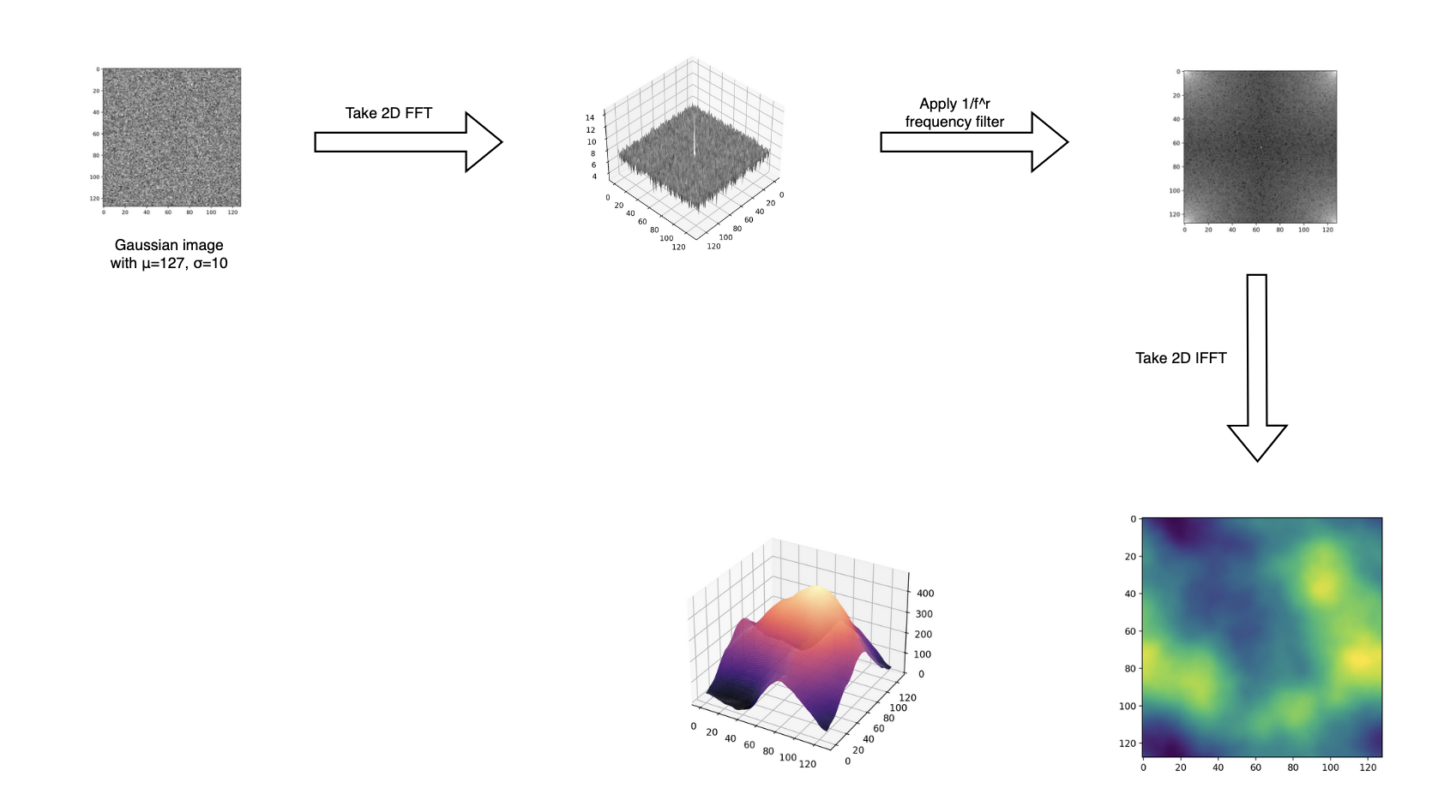
The high-level process for our system is outlined in the block diagram below (Figure 1). We first start with an image which has pixel values that are normally distributed. The result is then fed into a 2D FFT, after which each pixel value is scaled according to \(\frac{1}{f^{r}}\), where r is called the "roughness" parameter. Values close to 1 yield a more jagged landscape, while higher numbers result in smoother ones. We found that numbers around 2.5 produced the most natural results.
After all the calculation finished on the FPGA, the data was sent over to the HPS to be displayed on the VGA screen. Calculations for perspective, lighting, and control were all done in the C code. Threads and helper functions were created for this task.
Detailed Design
Initial Steps
FFT
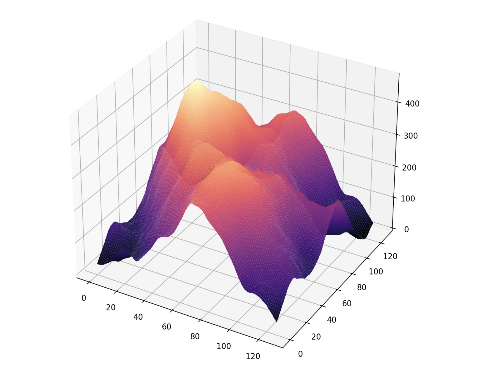
Before attempting to create a design which was implemented in hardware, we first focused on getting a simple program running in Python using pre-written FFT functions to achieve the desired landscapes as a proof of concept. Below in Figure 2 is a sample of a 128x128 landscape generated by our Python program, since it seemed that not many people had supplied code examples online which we could play around with.
We decided that a good next step would be to go slightly lower level and attempt to create the same program in C, but with our own FFT, IFFT, and frequency filter functions. The algorithm used was the Cooley-Tukey FFT algorithm, which breaks the FFT of a large signal into the sum of a bunch of smaller FFTs. This was extended to 2D signals by first taking the FFT of all of the rows, then on all of the columns, applying the frequency filter on each element, and subsequently taking the IFFT on each row and column.
The C program also did all of the computation using 20.7 fixed-point arithmetic. Since the input image will have values that range from 0-255, we determined that we would need at least 16 integer bits for just the FFT alone. We decided to add 4 more bits to this to allow for headroom to prevent overflow for other manipulations sucha as the frequency filter. We also decided that 7 bits should be fine for the mantissa, since we are not necessarily after high precision when creating graphics for landscapes given that we are already starting with a randomly distributed image to make an irregularly shaped graphic. Additionally, we chose the 27-bit width because the FPGA can directly use DSP blocks to speed up multiplications.
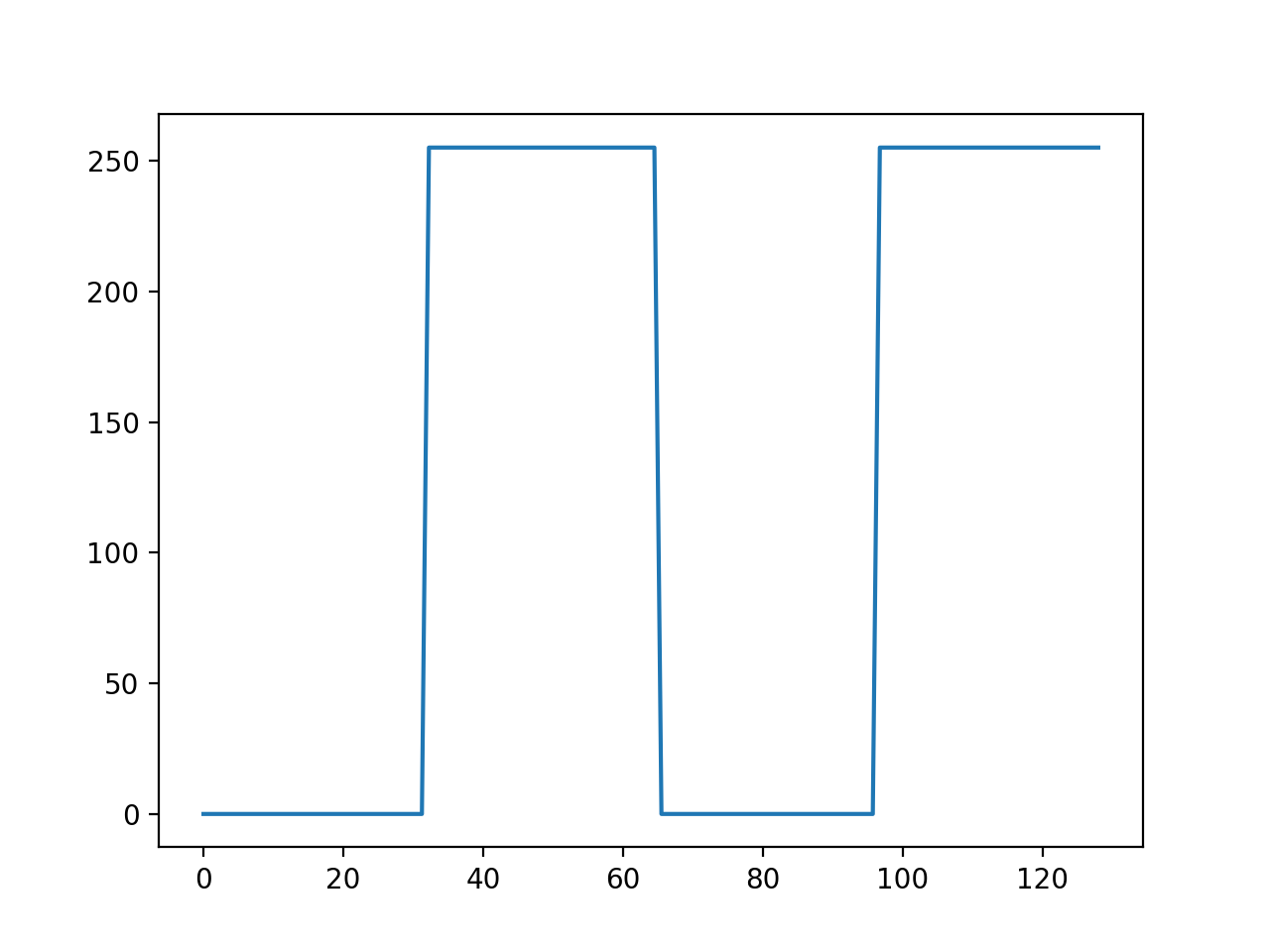
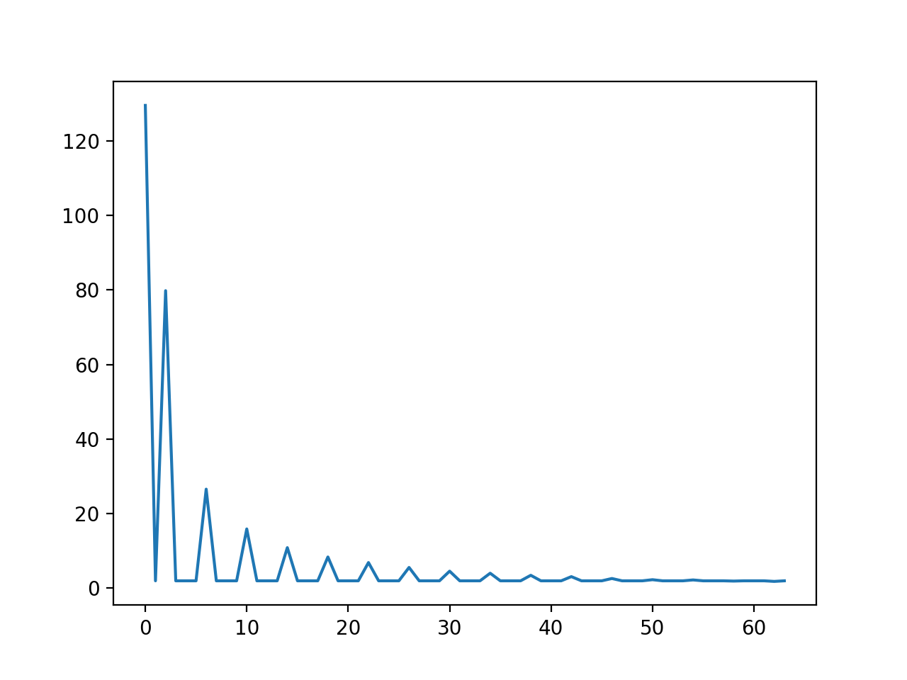
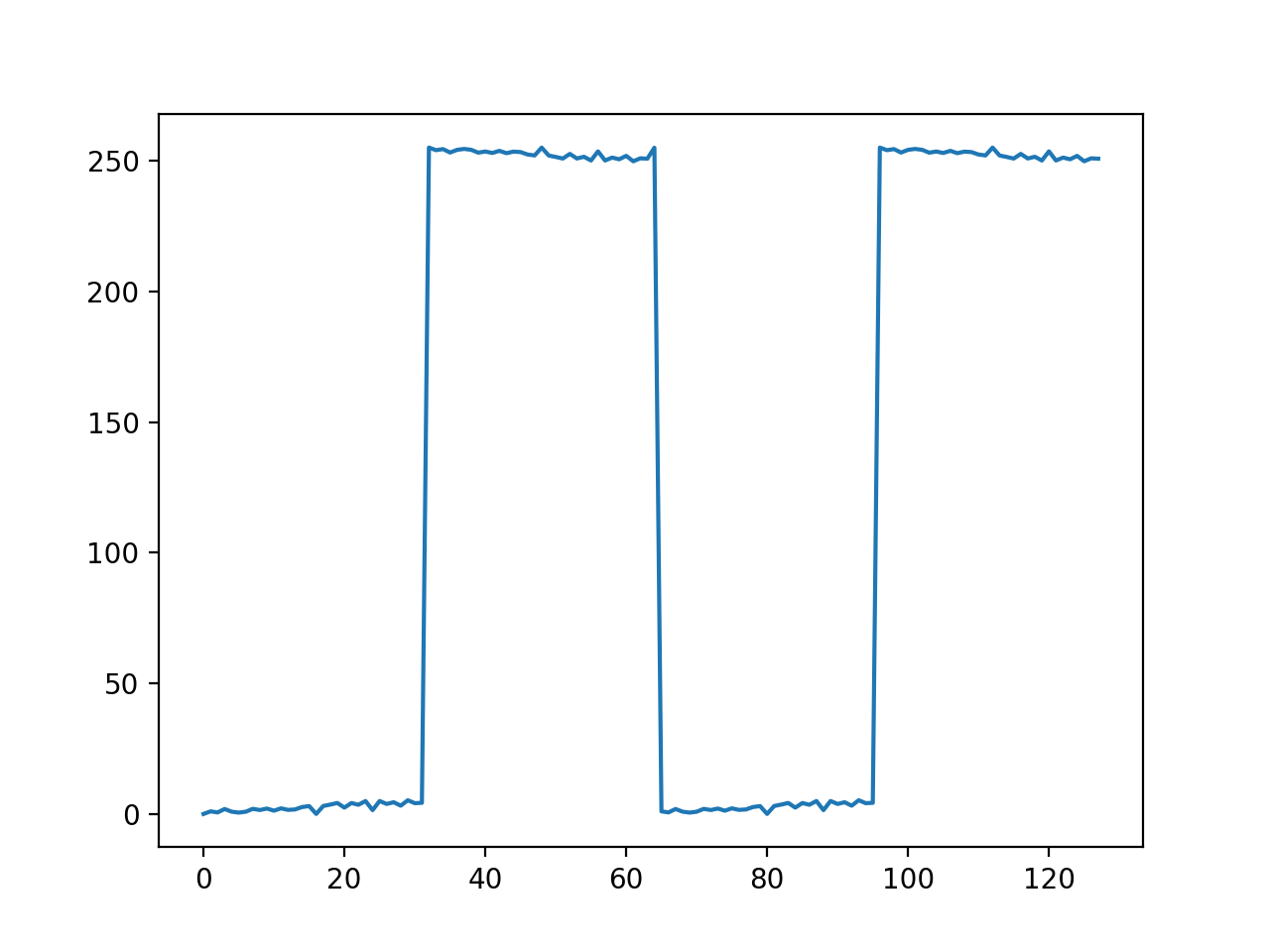
To test the C implementation, we input into the FFT a period and a half of a pulse train with a duty cycle of 50% (Figure 3). To verify that the output was correct, we knew that the frequency signal should have peaks in the 0th, 2nd and 6th bins with an exponential fall-off in magnitude (Figure 4). To verify the IFFT, we ran the result of the FFT through the IFFT and expected to get the original signal back (Figure 5). The ripples seen on the result of the IFFT can be attributed to the limited 7-bit resolution after the decimal point.
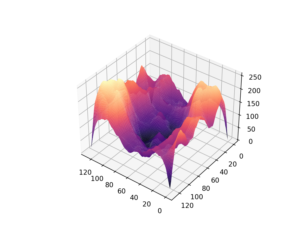
Once this was working, we moved on to trying to generate landscapes using the IFFT and FFT functions. This involved taking the transpose of the real and imaginary parts of the image after finishing the FFT or IFFT on each row in order to perform the operation on each column. The results for a 128x128 input image are shown in Figure 6. The coloring and visualization was done in Python.
Graphics
To better understand basic graphics principles, a Python implementation of a small 4x4 step mountain was created, complete with controls for changing the apparent distance and orientation of the object.
To render a 3D object onto a 2D screen, a series of matrix calculations must be done. Luckily, the NumPy library made the implementation relatively simple. First, a camera coordinate system was defined. This was created based on the camera position (defined to be (5, 0, 3)), the target point (defined to be (0, 0, 0), i.e. the center of the base of our object), and an "up vector" (defined to be (0, 0, 1), which is "up" from the camera's viewpoint). The view vector is defined as the unit vector pointing from the camera position to the target point. A perpendicular unit vector is generated by taking the cross product of the up vector and the view vector that was just calculated, then normalized. Finally, the coordinate system is completed by taking the cross product of the two perpendicular vectors. The camera view matrix is created by matrix multiplying a translation 4x4 matrix, which is a diagonal matrix of 1's except for the last row whose first three entries are the camera's position, with a rotation 4x4 matrix, whose entries are the vectors that comprise the camera coordinate system and a [0, 0, 0, 1] column vector at the end.
Next, a perspective mapping matrix is defined. Multiplying by this matrix, shown below, transforms the view volume (in our case defined with n as 4, f as 10, and h as 0.7) into a cube.
\[\begin{bmatrix} n/h & 0 & 0 & 0 \\ 0 & n/h & 0 & 0 \\ 0 & 0 & f/(f-n) & 1 \\ 0 & 0 & -(n*f)/(f-n) & 0 \end{bmatrix}\]The camera view matrix is matrix multiplied with the perspective matrix to form a final transformation matrix that is applied to all of the vertices in the object. These vertices are defined in the world coordinate system, the base of the mountain being centered at (0, 0, 0). Finally, perspective division is done to make the rendering seem more realistic by making points in the distance closer together.
To display the mountain, triangular faces are used. A 2d list of vertex indices corresponding to each face is defined using a helper function. This list of faces is iterated through, and each vertex is plotted. The camera height is adjustable, done simply by changing the z coordinate of the camera position. The mountain's apparent angle of rotation is also adjustable. However, instead of rotating the object directly, which would have been more complicated, the camera was moved instead, according to the equations below. This resulted in the same object rotation effect being produced.

A new transformation matrix is created as a result of these changes in camera position, and the new vertices of the mountain are formed and displayed.
A helper function for converting HSV color values to RGB was also written. Though this function wasn't used in the Python implementation, it served as a good tool for checking against while writing the C code for graphics.
The Verilog Code
A large amount of the development in the Verilog code was done in ModelSim to ensure that the foundations of the hardware were correct. Our initial goal was to take the FFT and IFFT and make sure that their implementation in Verilog produced the same output as the FFT and IFFT in the C code given the same input.
One important consideration that we had to make when designing the FFT in Verilog is that modules cannot use unpacked arrays an inputs or outputs. Therefore, each input into the FFT or IFFT needs to be a packed array of size (# elements)*(bit-width)-1. In order to carry out multiplications in fixed point, we also had to create a 27-bit multiplier module similar to what we made in the labs.
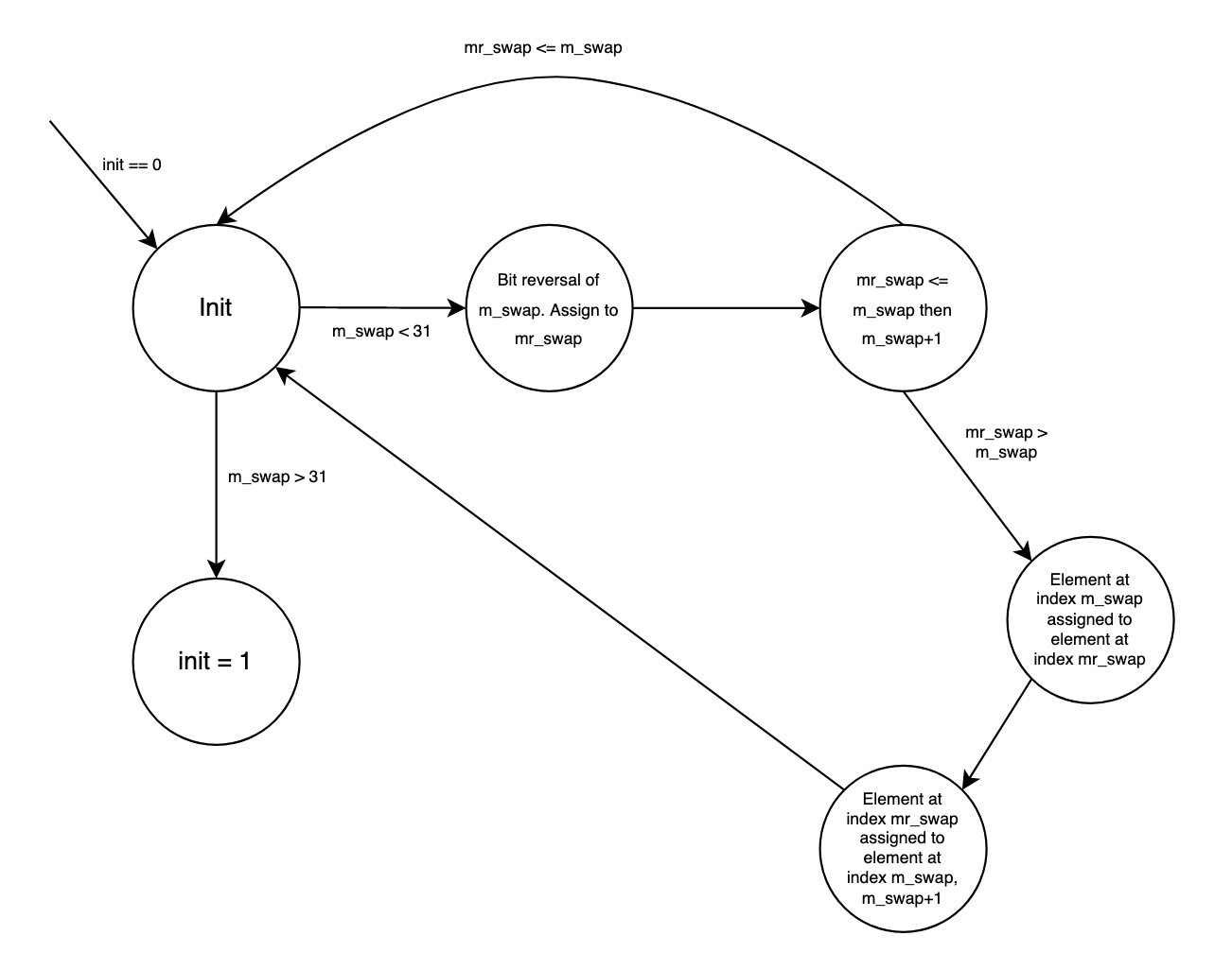
The FFT module contains two main state machines for computing a 1-D FFT: the first takes care of reordering the elements in the input signal, while the latter actually computes the FFT. The initialization state machine reorders the input signal elements by keeping track of two indexes called m_swap and mr_swap, where mr_swap is just m_swap with the bits reversed. Then, the elements at index m_swap and mr_swap are swapped, and the process repeats until every element has found a new location in the signal. Figure 7 illustrates this process.
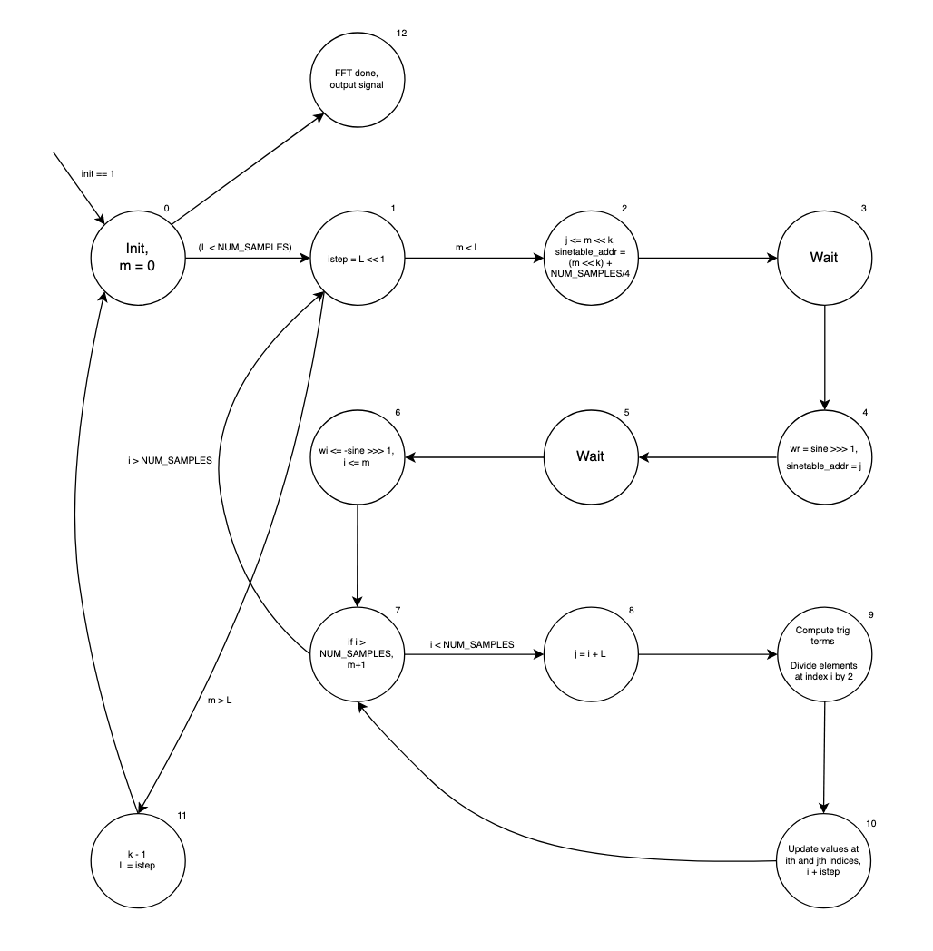
The subsequent state machine takes the reordered input signal which represents a collection of 1D FFT's and combines them to get higher point FFT's according to the formula in the High Level Design section. Moreover, this implementation uses a sin table as opposed to computing complex exponentials since it is much faster and less resource intensive to use a lookup table. In the state machine, i represents the index of one of the elements in the L-point FFT being combined to make a L*2 FFT, and j is the specific element being combined with i in a given iteration. States 2 and 4 do the necessary addressing into the ROM table, with state 2 fetching the result of the cos term and state 3 fetching the result of the sine term. State 9 takes the results of the multiplications of the trig terms with specific elements of the current L-point FFT signal from fixed point multipliers. Here, L is the number of elements considered in the FFT calculation, ranging from 1 (where the algorithm begins) to N. Finally, state 10 computes the new values at specific indices for the L*2 point DFT.
The method by which we tested the correctness of the FFT implementation was to input the same pulse train signal that was input into the C program, and make sure that the output was equivalent.
The IFFT is exactly the same as the FFT with just a couple very small changes. First, the sine term from the lookup table is not multiplied by -1. Second, the results from the lookup table and the elements of the L-pt FFT at the ith index are not divided by 2. To test that these modifications actually worked, we ran the output of the FFT we verified in Verilog through this IFFT, and made sure that the output matched what the output was from the C program (Figure 5).
As mentioned earlier, extending the 1D FFT to a 2D scenario is relatively straightforward. It is obtained by taking the 1D FFT of each row in the 2D signal, and then taking the result from that and calculating the 1D FFT on all of the columns. Since we can't directly pass the columns of the 2D signal through our FFT and IFFT module, we needed to create a way to transpose the 2D signal. Our initial plan was to have this done in a single cycle in Verilog, but complications with fitting the design onto the FPGA and ALM usage led us to move this operation to the HPS.
The Top Level Verilog Module
The top level Verilog module made use of SRAM to read and write each row of the image. In order to store the rows of the Gaussian image to the registers, we had to make sure that the HPS had finished writing the row to the SRAM. This was checked by the flag comp_ready against the previous comp_ready flag. If they were the opposites of each other, meaning that the value of comp_ready had been changed by the HPS, the image registers could start being initialized.
We created a state machine to read and write to the SRAM. In the first state, sram_write was set to 0, and the address was set to the column. Then there was a wait state for the data to be read from the SRAM. In the third state, the SRAM values were put into signal registers, by splicing into the registers as follows:
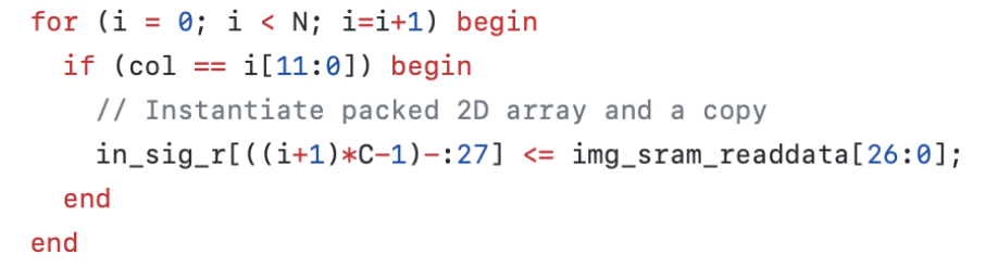
We stored both the imaginary and real parts of the image in the same SRAM. The next part of the state machine took care of reading from the imaginary part of the numbers, whose address was the column number plus 1024. Using the same register splicing shown above, the imaginary values were put into the register in_sig_i. Once all the cells in a single row were put into the corresponding registers, the FFT process could begin. We first checked that the do_fft flag was set to 1, and then reset the 'col' register to 0. In order to trigger the FFT, we set the fft_trig flag to be 1. If fft_trig was equal to 1, the FFT state machine could begin. In this state machine, we passed the in_sig_r and in_sig_i registers into the FFT module, and set them to the outputs of the FFTs.
Once the FFT was complete for one row, we created a new state machine to write the values back to the SRAM. In this state machine, we first specified the address and then wrote both the imaginary and real registers back into img_sram_write_data (the imaginary data was stored in the address of col+1024). Once the writing was complete, process_done was set to the opposite of what it was before, and comp_ready_prev was set to the value of comp_ready.
The IFFT was done in a similar way. If the IFFT was ready to be done (the do_fft flag was set to 0), ifft_trig was set to 1 and the signals were passed through the IFFT module.
QSYS
In order to complete our project, we had to add a few ports to our QSYS file.
process_done was a PIO port that would let the HPS know that the write back to the SRAM was done. It was set to the opposite of what it originally was once one row of the image was written back. The HPS could use this flag to wait until the row's FFT was done before moving on to the next row. The do_fft PIO port let the FPGA know if it was time to do the FFT or the IFFT. The comp_ready PIO port let the FPGA know that one row of the image had been written to SRAM, so it could start computing the FFT. Other PIO ports that were generated in the QSYS file were the reset ones. The hps_reset PIO port was connected to the second button (KEY 1) on the microcontroller, and would reset the HPS graphics. The seed generation reset was set to the third button (KEY 2) on the microcontroller, and this would restart the program with a new seed, so a new random Gaussian image could be generated.
The SRAM was also implemented through the QSYS on the heavyweight bus. As mentioned earlier, the SRAM was populated by both the HPS and the FPGA. Before any drawing happens to the VGA screen, the FPGA and HPS communicate through the shared block of SRAM to create the final landscape image. Each row of the initial Gaussian image is sent over to SRAM to the FPGA to calculate its Fourier transform. When the FPGA is done with the row, it writes it back to the appropriate space in SRAM, sets a flag, and the HPS reads the numbers back into an array. Once all of the rows are traversed, the HPS transposes the matrix and feeds the values back into SRAM for the FPGA to compute row-wise FFTs. This completes the FFT part of the process, and the HPS carries out the frequency filter on the image next. This filter multiplies each number in the current image by \(\frac{1}{f^{r}}\). Frequency bins are easier to think about for 1D signals given a sampling rate, but for images there exist spatial frequencies along the x and y axes. To get these frequency bins, we followed the definition that the numpy function fftfreq follows, shown in Figure 9.
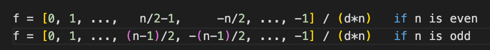
Here, d is the sampling period which is set to 1 in order to avoid going beyond the available decimal resolution of 7 bits. We generated two 32-element arrays to hold the frequency bin values on each axis according to the above formula. Then, for each element in the image array, we interpret the frequency value at a specific pixel location as being the square root of the sum of the x frequency at the column index squared and the y frequency at the row index squared, or: $$frequency[row][col] = \sqrt{xfreq[col]^{2} + yfreq[row]^{2}}$$ for a pixel at location row, col. Once the filter is applied to the image, the process to carry out the IFFT with the FPGA follows the same process as with the FFT.
Additionally, once the final image comes out of the IFFT, the values are not in an appropriate range to use to directly display on the VGA screen (some are negative, or too large). Therefore, the HPS scales the image to map each value to fit between 0 and 150 using the min and max values in the image according to the formula: $$new value = ((old value) + |min|)*\frac{150}{max + |min|}$$
The HPS
The C code uses multithreading to generate a landscape and do all the graphics calculations and control.
Landscape Generation
At first, we only wanted to have the HPS do all the graphics, shading, etc. However, after some trial and error, we realized that it wasn't possible to do the entire FFT, IFFT, transpose, and frequency filter in Verilog. Instead, we decided to have the HPS write one row to the SRAM, have the FPGA do the FFT, and repeat the process until the full FFT was done.
The landscape generation is in a thread called make_landscape(). We first checked whether Key 3 was pressed, which meant that the user wanted a new landscape to be generated. Initialization of the normally distributed image isn't as trivial as it is in Python, as there is no built-in funciton in C to get a number drawn from a normal distribution. Therefore, we created a function to do so which is called in main before any execution is done to compute the landscape according to the algorithm below:
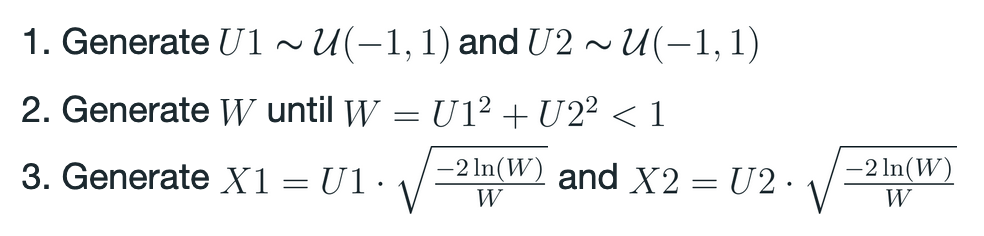
The algorithm approximates a Gaussian distribution by iteratively calling the rand() function that is included in the C standard library and which is uniformly distributed.
The 'ready_pio' flag was set to 1 once the first row of the Gaussian image was created, signaling to the FPGA that it could start reading from SRAM. do_fft was also set to 1, signaling that it should do the FFT, not the IFFT. We then waited until the fft_done PIO port was set to the opposite as previously was, meaning the FPGA had completed the FFT. This was done for each row of the Gaussian image.
Once the entire FFT was completed, transposes were done on the real and imaginary parts. The FFT was completed and the image was transposed again. After the second transpose, the frequency filter was implemented. Once this was completed, the IFFT process was started. This was completed exactly as the FFT was, but do_fft was set to 0, so the Verilog would set the IFFT_trig flag to 1, and start the IFFT. The same process as before (transpose, IFFT again, and second transpose) was completed again.
Graphics
The graphics portion of the C code follows the Python implementation fairly closely, with different values due to the increased size of the landscape, such as the camera being placed farther away. Unfortunately, all of the matrix calculations had to be done manually in the draw_vga() thread without the help of a convenient library like NumPy. One task that this thread does that the Python version does not is convert the coordinates into screen coordinates by scaling and shifting the transformed coordinates, and finally casting the value into an int to be output to the VGA display. Another feature added to this function was shading by implementing depth cueing. This technique makes points on an object that are farther away from the viewer appear dimmer, and it was modified in our code to also factor in the distance away from the light source. The HSV color model was used for shading, because the value of "value" directly affects how bright or dim a color looks. This thread's contents only run if any graphics parameters were changed by the user to prevent flickering on the screen while nothing else is happening.
Helper functions were defined and used to assist in the graphics rendering. One is the face list function that was also in the Python implementation, used to generate a list of vertices corresponding to each triangular face of the landscape. Another is a vertex list function. This was needed in the C code because manually defining each vertex was no longer feasible due to the size of the landscape (32x32 as opposed to 4x4), as well as needing to populate the z-coordinate column with the output of the FFT calculations done by the FPGA. Finally, a function for converting HSV to 16-bit RGB was written so that the VGA screen would display the color properly.
For graphics control, a thread called mouse_output() was created to transform the landscape's orientation and lighting. Moving the mouse left and right changes the location of the light source, while clicking the left and right mouse buttons rotates the landscape. An additional thread called check_reset() resets all of the graphics parameters back to the default if KEY 1 has been pressed on the board.
Results
Demo
In the end, we were able to create relatively realistic looking 3D landscapes displayed on the VGA screen using a wireframe construction and a 32x32 grid. A short video flipping through some of the generated landscapes is shown below.
Our initial approach was to have a grid of 128x128 points, and have FFT's running in parallel for each row, so that the FFT of the whole grid would take just twice the time to compute a 1D FFT. We quickly found out, however, that this exhausted the DSP blocks being used as well as the available ALM's. Each FFT and IFFT module in a generate statement uses 4 multipliers, meaning at most we could do 10 rows in parallel. Additionally, it seemed that having so many for loops and generate statements used to attempt to parallelize computation quickly used up the ALM's on the FPGA and resulted in hour long compile times which ultimately failed in the fitter stage. Even when we reduced the number of rows computed in parallel to 2 and the grid size to 32x32, the inclusion of the generate statements and for loops used to generate repeated hardware caused an excess use of ALM's. Additionally, with the final implementation, increasing the grid past 32x32 (while staying a power of 2) causes the fitter in Quartus to fail due to routing issues despite being well under the maximum allowed memory, ALM's, DSP blocks, and registers.
Conclusions
In conclusion, this project gave us a new perspective on how a random Gaussian image can be transformed into a natural-looking artifact. By putting it through a FFT, frequency filter, and then an IFFT we were able to demonstrate a maountainous landscape. We were able to successfully implement the FFT and IFFT in verilog, and make use of the SRAM to send and receive each of the rows of the image to/from the HPS. Finally, we were able to use C code to give the landscape depth through lighting and shading.
With more time, we would have liked to implement more advanced rendering and shading techniques such as scanline rendering and z-buffering to create more solid-looking mountains. Casting shadows from the peaks of the mountains onto lower parts of the mountain according to the location of the light source would have been interesting to see done as well. Another area in which our design could improve is with optimization of the FPGA side so that as much computation of the landscape can be done there as possible instead of just having the FFT and IFFT there. This would involve thinking more carefully about how the design could better fit within the resource constraints of this particular FPGA while being able to maximize what is computed in parallel. However, we are still extremely proud of what we were able to accomplish with this project.
Appendix A: Permissions
The group approves this report for inclusion on the course website.
The group approves the video for inclusion on the course YouTube channel.
Appendix B: Code
Full Verilog Project
Top-level Verilog Code
FFT Verilog Code
C Code
FFT Python Test Code
FFT C Test Code
Graphics Python Test Code
Appendix C: Member Contributions
Jenny Wen: All things graphics (Python, C) and website format
Luis Martinez: Verilog, HPS-FPGA communication, Python FFT test script, and C FFT test program
Aratrika Ghatak: Verilog and HPS-FPGA communication
Appendix D: References
Professor Land's Graphics MATLAB Code: GUI and Function
Professor Adams's Cooley-Tukey FFT Guide: Understanding the Cooley-Tukey FFT
Fractal Landscape PPT by A. Krista, Bird B. Thomas Dickerson, and C. Jessica George: Techniques for Fractal Terrain Generation
Gaussian Distribution Generation: Generating random numbers from Normal distribution in C