By Stefen Pegels(sgp62), Ruby Min(rbm244), Hannah Goldstein(hlg66)

Introduction

For our final project, our goal was to produce visually appealing and organic-looking landscapes that may be used in computer graphics applications. We decided to implement the diamond-square algorithm to procedurally generate terrains by producing heightmaps in hardware on the FPGA. The generated terrain is shown on the VGA display, and a user can change settings to create different looking terrains with different features (sand, snow, water, land, greenery, etc…). Our original aim was to optimize both th e size of the landscape generated as well as the speed at which the entire height map is generated. While we did initially parallelize the algorithm using hardware resources, we decided to sacrifice some speed in favor of having a larger map and ultimately ended up being able to display 257x257 terrains on the VGA screen with an unperceivable update rate. Still, the total calculation of the 257x257 height map is about 30 times faster than a Python simulation, even without parallelization.

High Level Design

Diamond-Square Algorithm Overview

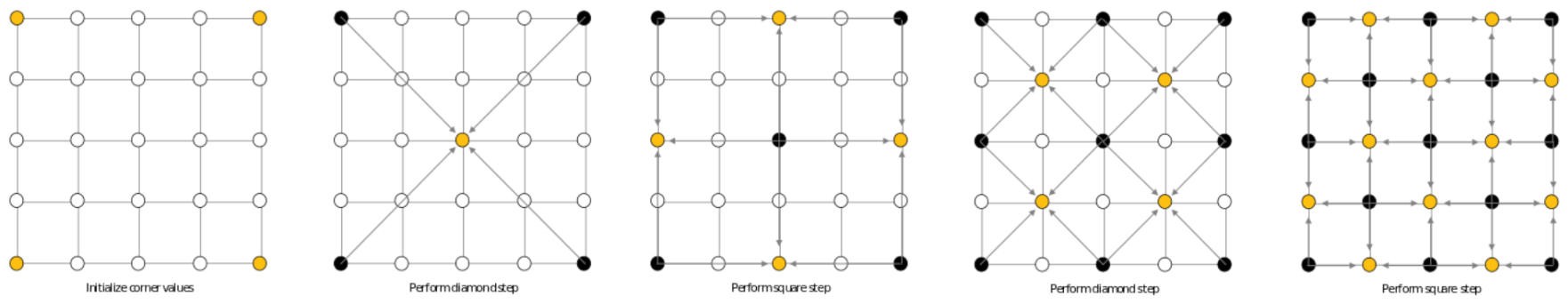
Figure 1: Diamond Square Overview, taken from http://jmecom.github.io/blog/2015/diamond-square/

The diamond square algorithm starts off with a 2D square grid of dimensions 2n+1 by 2n+1, where n is a positive integer. The four corners are initialized to some set of values (we decided to make them user inputs in our implementation). Below, we will follow the example of a 5x5 grid.

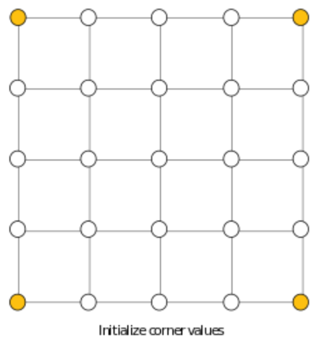
Figure 2: Corner initialization step

Then we perform the first “diamond” step. We look at every square in the grid formed by the points in the array that already have values (black point in diagram below), find the center point (yellow point), and calculate a value for that center point by taking the average of the four corners plus some random value.

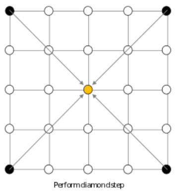
Figure 3: First Diamond Step

Next, we perform a “square” step. This involves taking all the diamond shapes formed by the points in the grid with values (black points), and then calculating values for their center points (yellow points). The value is once again calculated using the average of the four corners plus a random value.

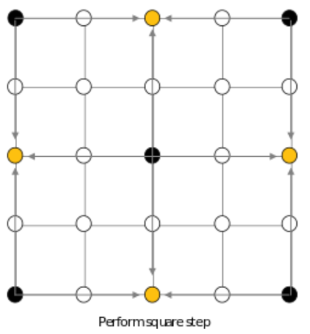
Figure 4: First Square Step

These diamonds include ones that wrap around the side of the grid. For example, the leftmost diamond has a “missing” leftmost point as shown below. We decided to use a wrap-around method for these boundaries, and so the fourth value missing would be taken from the other side (although in this step it is the middle point again).

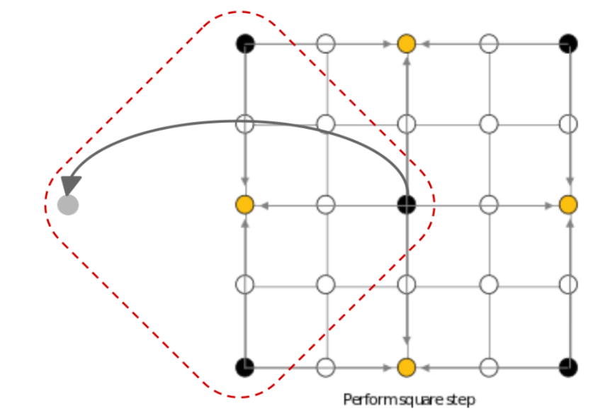
Figure 5: Demonstrating wrap-around value using in square step

Then, we repeat the diamond step with the new grid (essentially at the next depth), and then the square step until all points on the 2D grid have a value which is the height at that point. Here is the rest of the 5 by 5 grid example (again showing an example of the wrap-around in the square step):

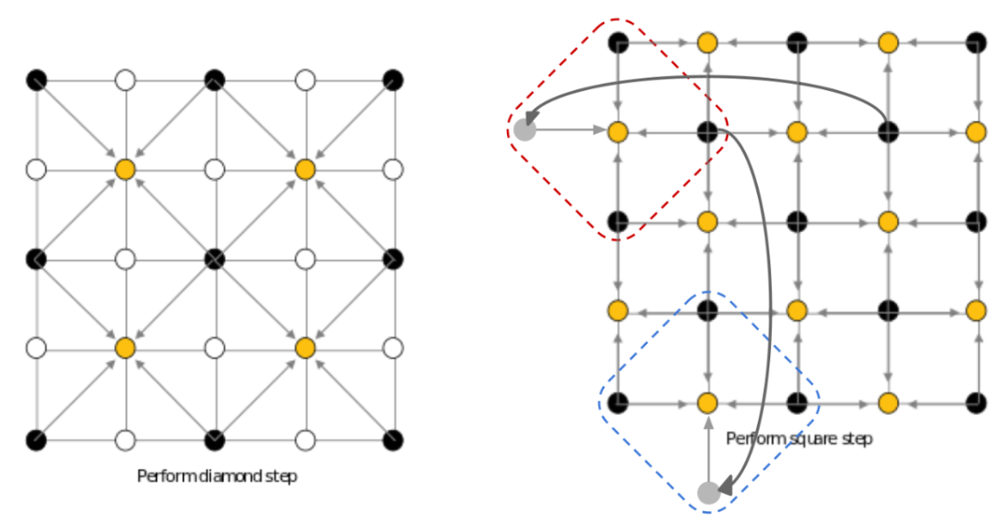
Figure 6: Final diamond (left) and square (right) step for 5x5 grid

For the general 2n+1 by 2n+1 grid, we perform a diamond and then a square step a total of n times to fill the entire grid. Note that the range that the random value (added to the average calculation) is chosen from decreases with every set of diamond-square steps to generate more continuous mountainous terrains.

HPS and FPGA High-Level Design

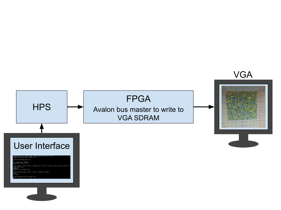
Figure 7: Project Hardware Setup

The overall design for our project consists of the HPS (with the user interface), the FPGA, and a VGA display screen. On the HPS, we generate a simple command line interface from which a user can change a variety of settings. These include the initial values for the four corners, the seed for our pseudo random number generators (more details in the Hardware Design section below), as well as the type of terrain to be displayed (swamp, desert, arctic, volcanic, or islands). These are sent to the FPGA through PIO ports as detailed below. On the FPGA, we have our hardware implementation of the actual diamond square algorithm to generate the height map. On the FPGA is also the implementation for writing the final pixel colors to be displayed on the screen (by writing the VGA SDRAM through an Avalon bus master). For the display, we color the pixels (points on the grid generated by the diamond-square algorithm) based on altitude. Each type of landscape has a different set of colors and altitude ranges for coloring.

Hardware Design

Translating Diamond Square to the FPGA

To initially lay out the diamond square algorithm to get a sense of its steps, we implemented it in python. The translation to Verilog required a state machine to move through the Diamond and Square steps, combined with M10k memory storage for each column of the map. Since the DE1-SoC caps at ~390 M10k blocks, and the Diamond Square algorithm requires map dimensions of (2n+1, 2n+1), our largest map would be (257,257).

Initially we attempted a parallel approach where separate solvers would fill their own M10k block and pass values to adjacent columns, but we ran out of ALMs with this approach (maxing out at a 33x33 map). Our final implementation was a serial solver that executed parallel M10k reads and computed the values one at a time. The RTL for this single solver can be found here . The state machine for this implementation took the following shape:

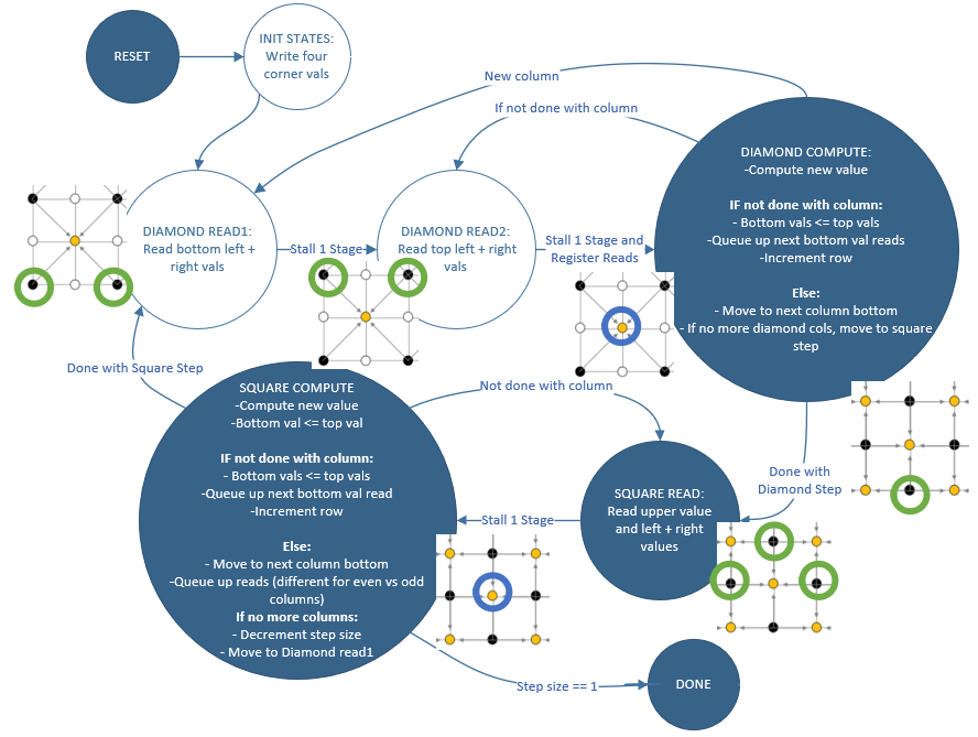
Figure 8: Single Solver State Machine, with illustrative images to show reads (Green) and writes (Blue) at specific steps

Illustrated by the above diagram, the single solver moves back and forth between the diamond and square steps, performing all of the diamond step calculations for all rows/columns at the given step size (depth), followed by all of the square step calculations for all rows/columns at the same depth. Each computation requires four reads to compute the weighted point average with added randomness for the altitude at a given point. Once all diamond and square steps are computed at this depth, the step_size decreases by a factor of two and the state machine is run again, eventually until all values on the board have been filled. Not pictured in the state machine diagram are specific stall stages for M10k read latency/register loading; only the algorithmic logic states are pictured. Once the step_size reaches 1 and the square step finishes, we have finished the entire board, and enter the done state, where the values are written to the VGA screen for display.

Communicating with the VGA Screen

Once the diamond square landscape grid is computed and stored in M10k blocks, we need a way to display the generated data onto the VGA screen, with relevant colors to properly display the landscape. Initially, we experimented with writing values directly to VGA synthesized SRAM, allowing one VGA write every cycle. However, this created issues when we attempted to scale up our maps to larger sizes since the VGA synthesized SRAM uses M10k blocks in addition to the columns of the generated map. To mitigate this, we implemented a bus master that writes to VGA SDRAM, trading slower VGA writes for more M10k design space. We saw this as a valuable tradeoff given that we weren’t designing for any speed constraints; we only considered area constraints for our design to generate the largest map. The process of writing to the VGA screen involves a bus master state machine and a state machine in the diamond square operator, working together to pass values to the VGA in the following manner, where both state machines stay idle until all M10k blocks are filled by the solver state machine, and begin once that finishes:

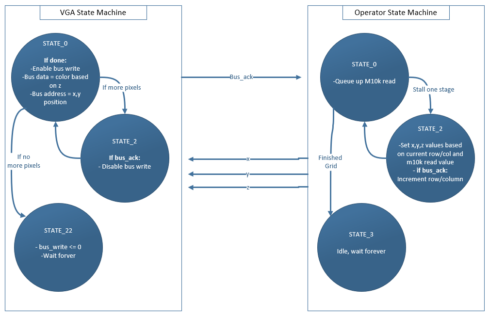
Figure 9: VGA Write State Machine working with Diamond Square Output State Machine

The operator produces the x,y (column,row) coordinates along with the z value (altitude) that was stored in the M10k block at that x,y position and outputs these to the top level module that reads them in. The VGA state machine uses the x and y position to create the SDRAM bus address, and the z coordinate is used to determine the color for the bus write data. We used 8 bit color for our landscape generation, and each landscape biome has 8 colors with their own altitude thresholds (see Software Design section). Once all of the SDRAM pixels have been written, both state machines stay idle until another reset. The RTL for the top level design can be found here.

Randomness with LFSR

When calculating the height for a given point on the diamond square grid, a random value is added to the four-point average from the adjacent points. In order to create randomness on the FPGA, we utilized a 64 bit Linear Feedback Shift Register with 16 bit output, which uses a set of XOR gates to create a spanning set of all values in the 64 bit space, with one new value shifted in every cycle as the output of the XOR function.

Figure 10: Example of a 16 bit LFSR

In our implementation, we take a random 32 bit seed from the HPS (See Parallel IO Ports section) and use this seed to create seeds for 16 other LFSRs. We then assign LFSR outputs to specific columns of the grid for use in that column’s random calculations. The 8 bit random number is added to the result of the 4-point average, accounting for overflow. Each time step_size decreases (meaning we move to a lower fractal depth), fewer bits of this random value are used in the four-point average, to create more homogeneity in the eventual landscape.

Software Design

Parallel IO Ports (QSys)

For this project, the HPS had a minimal role of generating random seeding and initial corner values for the grid, as well as switching between biomes and sending the corresponding color palette to the FPGA over a parallel IO port. Our Qsys setup for the project was as follows:

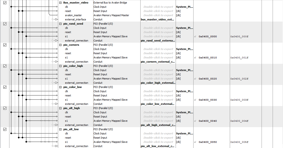
Figure 11: Qsys Declarations for Diamond Square Project

Notable on our Qsys bus was the Bus_master_video, which we used to interface with the VGA SDRAM and write our screen pixels. Important in our design for this bus master was the correct memory base for the SDRAM, which is listed at 0x0 in Qsys. This ensured we were writing to the correct memory locations with our bus master.

As mentioned in the Randomness with LFSR section, the random seed was passed as a 32 bit value which was duplicated as the input to the LFSR synthesized on the FPGA. The user also can change the initial corner values of the grid with the pio_corners port. For color and altitude, two 32 bit ports were used, with the color port partitioning the two ports into 8 separate 8-bit colors, and the altitude ports partitioning the ranges of altitude corresponding to those colors. For our 5 biomes (swamp, desert, arctic, volcanic, islands), the colors and altitude thresholds were as follows:

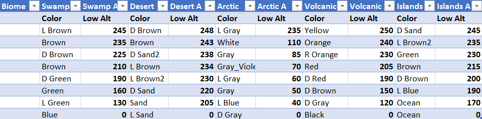
Figure 12: Colors per Biome and corresponding lower bound Altitudes for each

These 5 configurations were stored in 32 bit integers on the HPS, and the UI enabled selecting and switching between them; showing the altered biome with a reset on the FPGA as the color and altitude thresholds were passed over a PIO port to the FPGA. The FPGA reads this PIO input when selecting values for the color_reg which eventually becomes the SDRAM bus write data.

Color Selector Interface

During our demo and during testing of our system, we created a simple user interface running in MobaXTerm for configuring the landscape generation.

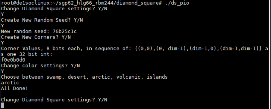
Figure 13: HPS User Interface for changing the landscape

This interface had three basic functions: setting a new random seed, changing the value of the four corners, and switching to a different biome. The user responses were captured with scanf from the command line. In the above image, the user creates a new random seed (0x76b25c1c), creates four new corner values (f0e0b0d0) where each set of 8 bits is one corner, and switches to the arctic biome. Each of these parameter changes is observable on the VGA screen after a KEY0 press on the FPGA.

Results

During the first week, we successfully implemented the algorithm using a small 5x5 sized grid, shown in Figure 14(left). Using fixed corners to initialize the algorithm, we were able to show that the system worked. We then embarked on creating larger grids and implementing randomness into the design. While an attempt to implement parallelism was made, we chose to go the route of serially writing the values to memory in order to maximize the size of the grid. During week two we focused on implementing larger grids and the LFSRs for pseudorandomness generation. We concluded the project by implementing several biomes by setting different colors and associated altitudes. Using inspiration from real-world images, we created five biomes - swamp, desert, arctic, volcanic, and islands. Because our project is heavily based on visual accuracy, our main metrics for analyzing the design come in the form of speed and visual fidelity. The progression of size increase as more optimizations and design decisions were made is shown in Figure 14.

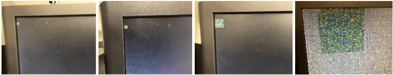
Figure 14: Rendered images of various grid sizes - from left to right - Grid of size 5x5, Grid of size 9x9, Grid of size 17x17, Grid of size 129x129

Comparisons between the Serial FPGA design and both the Python and Parallel FPGA designs can be made. The total time to complete a drawing for two grid sizes is shown in Figure 15. For a grid of size 33x33, the parallel implementation on the FPGA took 0.00456 ms, while the serial design took 0.06534. As a result, the serial design took 14.3 times longer to complete than the parallel design. While this performance increase may seem significant, this difference is indiscernible to the human eye. And, the parallel design required significantly more M10K blocks of memory than the serial design, and as a result, the parallel design could not render larger images. When comparing the serial design with the Python design, for a larger, 257x257 grid size, the speed benefit of our design becomes apparent. The Python design took 90 ms to fully render the 257x257 grid size, while the serial FPGA design took only 3.96 ms, meaning the serial design was about 22.7 times faster than the Python design. Therefore, while the parallel design was faster than the serial, the serial design, relative to a purely software implementation, offers a significant overall acceleration benefit.

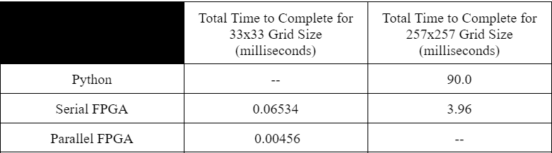
Figure 15: Speed performance of the three designs considered

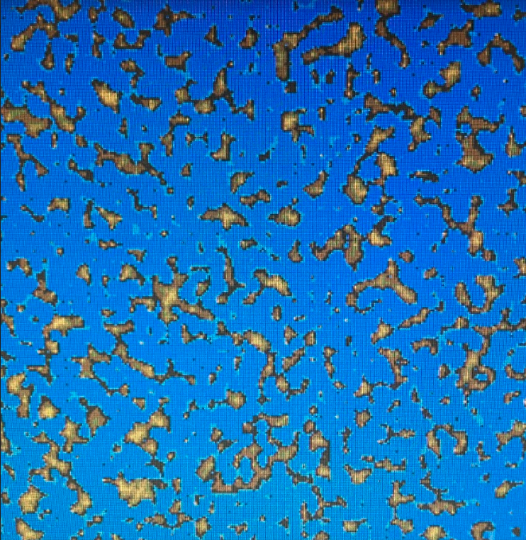
The second factor we wanted to consider was the appearance of the final design. Because the largest grid we were able to render, without requiring the use of SDRAM memory, was a 257x257 grid, we found that this often produced images that had a high level of variation. While this is accurate for some biomes, such as the desert and arctic, this proved to be less realistic for others, such as the swamp and volcanic biomes. As a result, we attempted to implement a further improvement on our design that caused four pixels, in the shape of a square, to map to each generated pixel on the FPGA side. This resulted in the images shown in the middle of Figures 16, 17, 18, 19, and Figure 20. WHile we were able to successfully implement this aspect of the design, we ran into a timing/ synchronization issue where switching between biomes would not fully complete after one reset. As a result, we had to press reset multiple times to remove any reminiscence of the previous biome. Because this issue could not be resolved, we opted to omit this design from the demonstration and include it here for reference to understand a possible route of improvement for our design. Below are five biomes represented through the maximum grid size that could be achieved with the serial implementation, the maximum 2x2 square per pixel implementation that was achieved, and the image that served as inspiration for the altitude cutoffs and coloring for the specified biome:

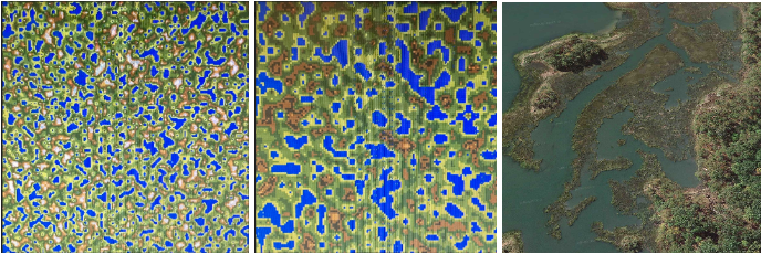
Figure 16: Swamp Biome - from left to right - 257x247 single pixel representation, 129x129 square pixel representation (using 2x2 squares of pixels for each one pixel calculated), image of the Marshlands Conservancy in Rye, New York ( 40.953611, -73.702222 )

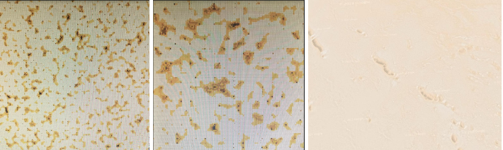
Figure 17: Desert Biome - from left to right - 257x257 single pixel representation, 129x129 square pixel representation (using 2x2 squares of pixels for each one pixel calculated), image of the Madigan Gulf in Australia ( -28.893112, 137.641166 )

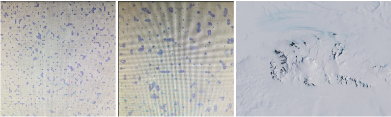
Figure 18: Arctic Biome - from left to right - 257x257 single pixel representation, 129x129 square pixel representation (using 2x2 squares of pixels for each one pixel calculated), image of Antarctica ( -80.700631, -29.624535 )

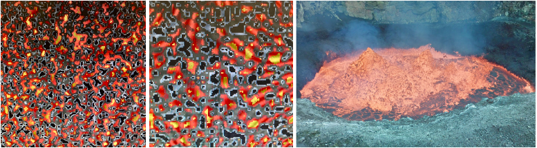
Figure 19: Volcanic Biome - from left to right - 257x257 single pixel representation, 129x129 square pixel representation (using 2x2 squares of pixels for each one pixel calculated), image of the Marum Crater Lava Lake on Ambrym Island, in the nation of Vanuatu

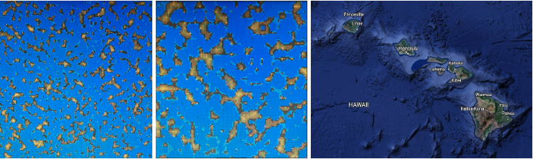
Figure 20: Islands Biome - from left to right - 257x257 single pixel representation, 129x129 square pixel representation (using 2x2 squares of pixels for each one pixel calculated), image of Hawaii ( 20.404418, -157.509103 )

Video

Conclusions

We successfully implemented the diamond square algorithm with color altitude limits to achieve the goal of producing a visually appealing, organic landscape for computer graphics in mind. By using the diamond-square algorithm, we were able to procedurally generate terrains through the creation of heightmaps on the FPGA. While parallelism was a consideration, we made the decision to forego this optimization to achieve larger map sizes. A user interface was implemented to allow the user to alter the settings to produce different biomes and different terrains within a specified biome. While this produced a slight speed decrease that was indescribable to the human eye, the overall performance, coupled with the maximum size our design could produce, was optimal relative to both the strictly software and parallel designs. This design decision allowed us to ultimately generate a large 257x257 map that could be produced at a speed that was visually acceptable.

Appendix A: Permissions

The group approves this report for inclusion on the course website.

The group approves the video for inclusion on the course YouTube channel.

Appendix B: Code

HPS (C) Code for this Project: https://github.com/sgp62/ECE5760/blob/main/FinalProject/DS_PIO.txt

Verilog Code for this Project: https://github.com/sgp62/ECE5760/blob/main/FinalProject/De1_soc_bus.txt https://github.com/sgp62/ECE5760/blob/main/FinalProject/ds_single_operator.v

Repository with Website Code for this Project: https://github.com/sgp62/ECE5760/tree/gh-pages

Appendix C: References

Reference for DE1-SOC base project: https://people.ece.cornell.edu/land/courses/ece5760/DE1_SOC/DE1_soc_computer/VGA_state_machine/DE1_SoC_Computer.v

Reference for diamond-square algorithm: http://jmecom.github.io/blog/2015/diamond-square/

Reference Images for Biome Inspiration were all obtained from Google Earth: https://earth.google.com/web/@0,-168.7112297,0a,22251752.77375655d,35y,0h,0t,0r

Appendix D: Work Distribution

Stefen: Wrote the Hardware Design and Software Design sections of the lab report. Hannah: Wrote Results and Conclusion sections of the lab report. Ruby: Wrote Introduction and High-Level Design sections of the lab report.

Everyone worked together collaboratively in lab for the implementation of this project.