Heat Diffusion Simulator
by Guadalupe Bernal (gb438), Nikitha Sharma (ns756), Frances Lee (fl296)
ECE 5760 Final Project Report submitted on May 18, 2023
Project Introduction
The goal of this project is to create an interactive heat diffusion simulation using the heat equation on a discrete domain, which allows the user to pick sources and sinks on the VGA screen and simulate the resultant reactions in real-time on the VGA screen.
To complete this project, we utilized the De1-SOC FPGA, a VGA screen, and a mouse, along with a robust hardware and software design. On the hardware side, our Verilog code utilizes hardware on the FPGA to generate a grid of cells, compute the thermal magnitude of each cell, select the respective color based on the magnitude, and plot the colors to the VGA. On the HPS side, our C++ code allows the user to inject heat on the VGA screen and to see the gradient-like visual effects in real time. We have one mode with preset sources/sinks and another mode with no sources/sinks. All together, we were able to utilize the knowledge and skills learned from our previous labs to build a beautiful simulation.
High Level Design
Initially, we wanted to model individual Monarch butterfly behavior patterns and how they flock together, as they are known for their unique migration patterns and ability to navigate through environmental conditions based on temperature. Given more extensive research however, there were no equations out there to model flight patterns, so we pivoted to simulating the thermal distribution given a variety of heat sources and sinks in spirit of our original project.
Background Math
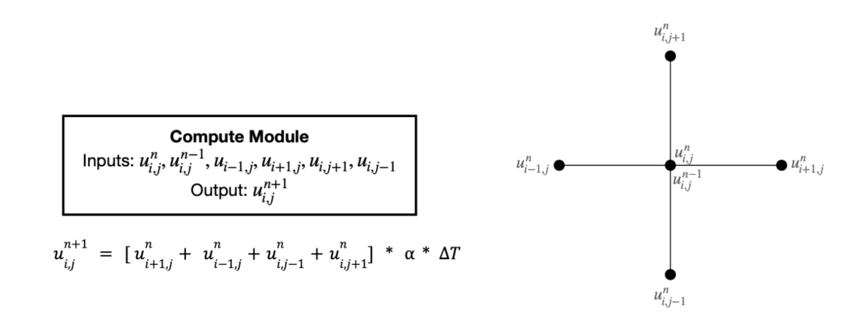
The discrete heat diffusion equation is a numerical approximation of the continuous heat diffusion equation, which describes the behavior of heat conduction in a given domain over time. To implement this equation on the FPGA, we used the discretized version, which breaks down the domain into a grid of discrete points and approximates the heat transfer between these points based on their neighboring values. The 1D discrete heat equation is expressed as the following:
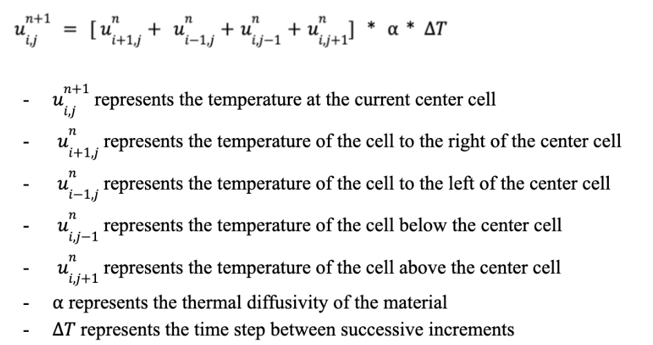
The equation calculates and updates the temperature at each point in the grid based on the temperatures of its neighboring points at the previous time step. For our design, we multiplied the alpha and change in temperature to control the rate of heat transfer between neighboring grid points in each iteration
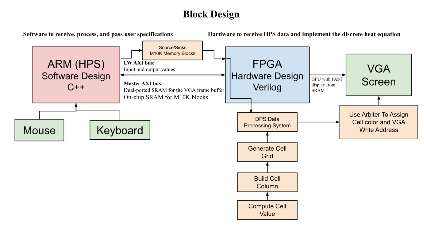
To solve the discrete heat diffusion equation, we start with either no heat or with an initial temperature distribution throughout the grid. Upon a heat injection, the design iteratively calculates the temperature at each point for subsequent time steps using the equation mentioned above. This process continues until the temperature distribution reaches a steady state. The block design that imlements our logical structure is shown below.
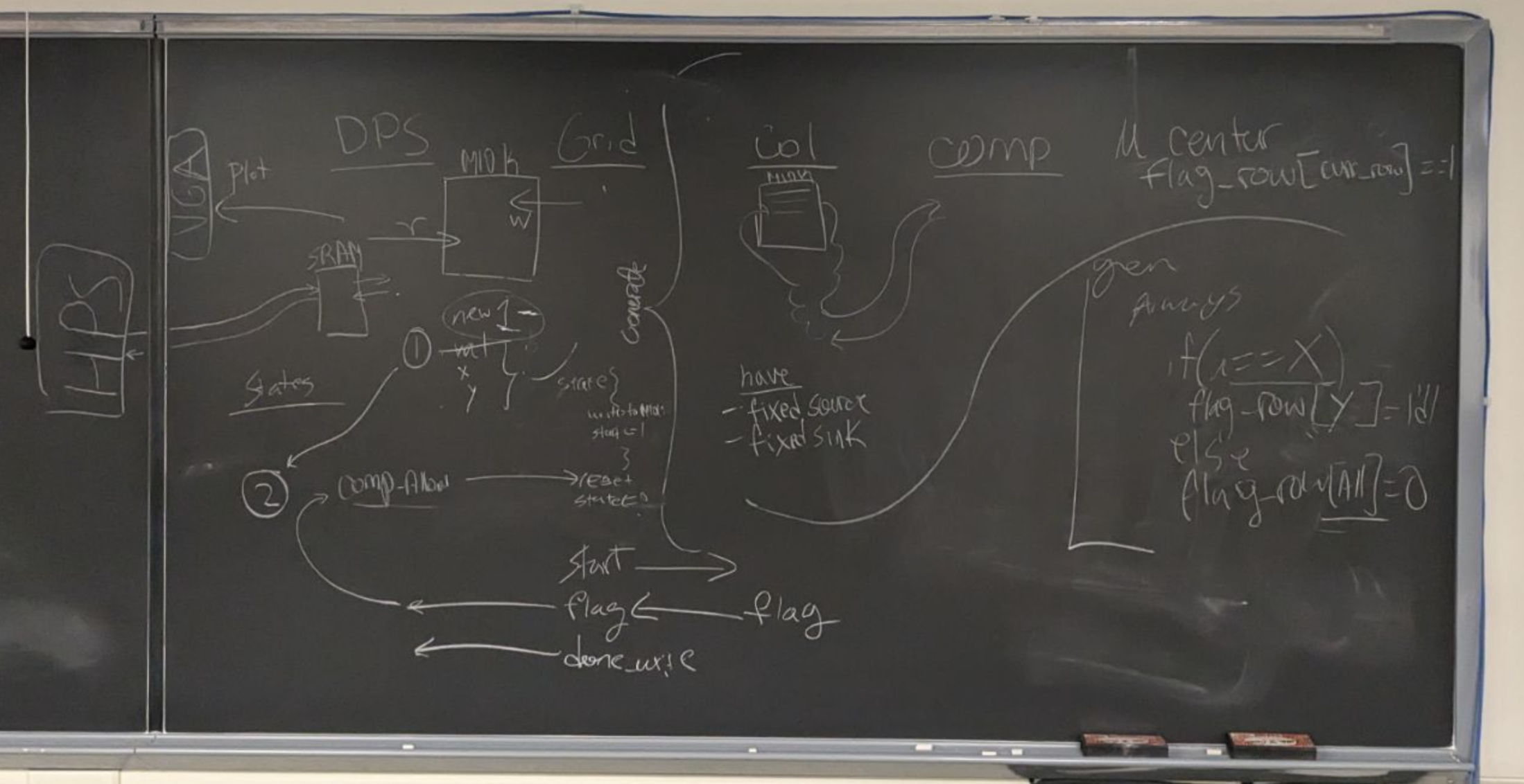
Logical Structure
As shown from the block diagram, our solution comprises four layers that work together to achieve the desired functionality. The bottommost layer is the compute module, responsible for determining the new temperature of each node based on inputs from neighboring nodes, the alpha and delta t constants.
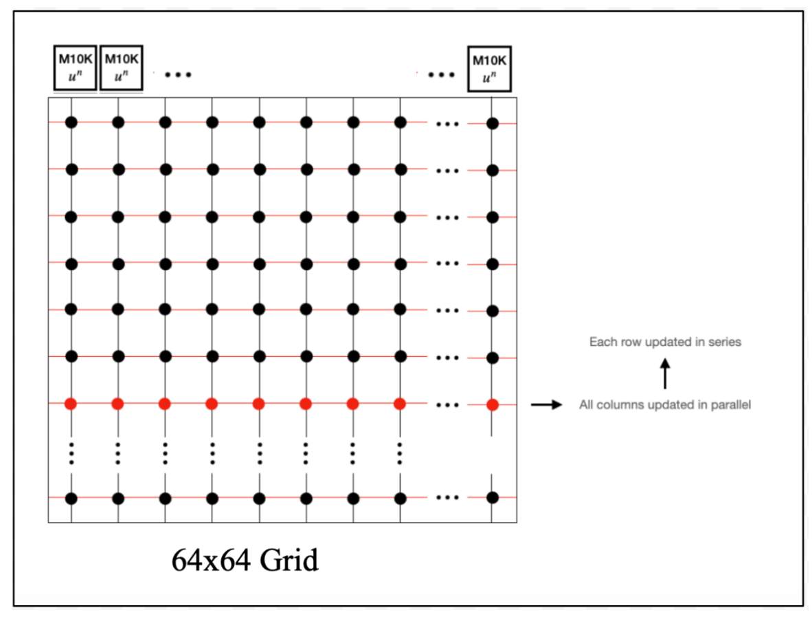
Above the compute module is the build column module, which constructs a column of temperature values. It iterates through all the nodes in the column, instantiating and utilizing M10K memory block for each column to store temperature values for each node.
The build grid module forms the layer above, handling the control signals necessary for advancing to the next column until all columns have computed their node values. A generate statement is used to generate the hardware for each build_column module and establish connections between left and right input values.
At the highest layer is the data processing system (DPS) module, responsible for data transmission between the HPS and FPGA. It updates values in the M10K memory and processes heat injection inputs from the user interface on the HPS. It reads the data values passed from specific SRAM addresseses and stores them in their appropriate M10K memory blocks based on the node's location. The DPS module also determines when to initiate the next iteration of grid calculation, and iterates through all the nodes to determine their pixel colors according to their temperature value and display them to the VGA screen.
Through the collaboration of these layers, our solution effectively handles the computation, storage, and visualization aspects of the heat diffusion simulation.
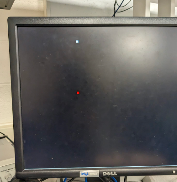
On the HPS side, we are running a program with three threads running concurrently. The first thread's purpose is to draw the cursor on the VGA screen and keep track of the mouse's location and user clicks. When a mouse click occurs, the x and y coordinates of the click are stored in an array for further processing. The second thread is responsible for passing the stored coordinates from the HPS to the FPGA using Qsys PIO ports. These coordinates are essential for the FPGA to perform relevant computations when updating the grid. The third thread handles keyboard input detection, allowing the user to indicate whether they want to perform a heat injection or create a heat vacuum. We focused solely on implementing heat injection functionality.
Software/Hardware Tradeoffs
Similar to the multi-processor drum synthesis lab, the FPGA framework for this heat dispersion project serves well for parallelization. Given that each evolution of the grid depends on the state of itself/values inside of it calculated from the previous timestep, we enhanced parallelization by walking up the columns and serializing memory sharing using the M10K memory blocks. Since most of the project is implemented in Verilog, there isn’t much software involved. We have used 64 M10K blocks for making the grid and an additional 2 M10K blocks (reading/writing data to SRAM from HPS to FPGA and reading/writing data for pixel color) to build our module. We made another tradeoff by using 32 bit values for the grids. If we used 18 bits, we would be able to leverage the fact that we have 18x18 multipliers on the board. We chose to do this because our color palette is extensive and we wanted to have a more precise range of values for the simulation.
Program and Hardware Design
C Implementation
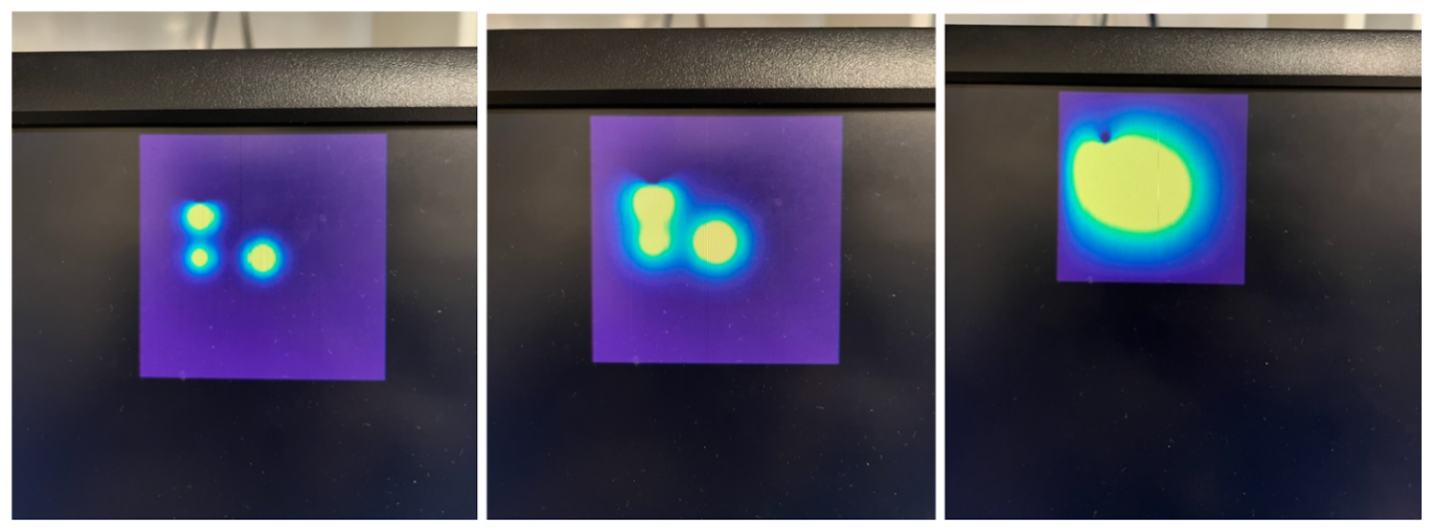
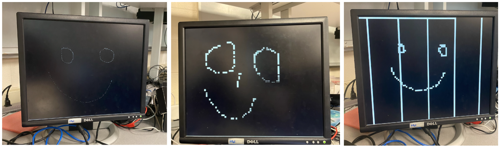
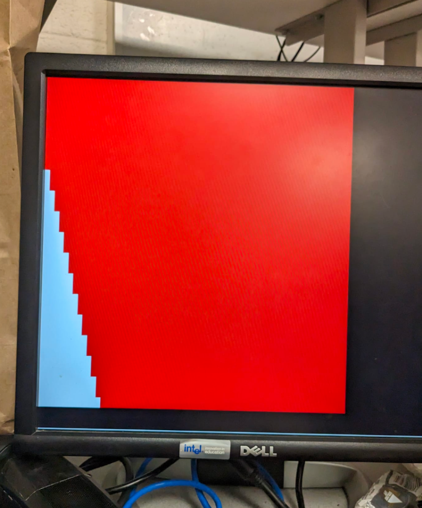
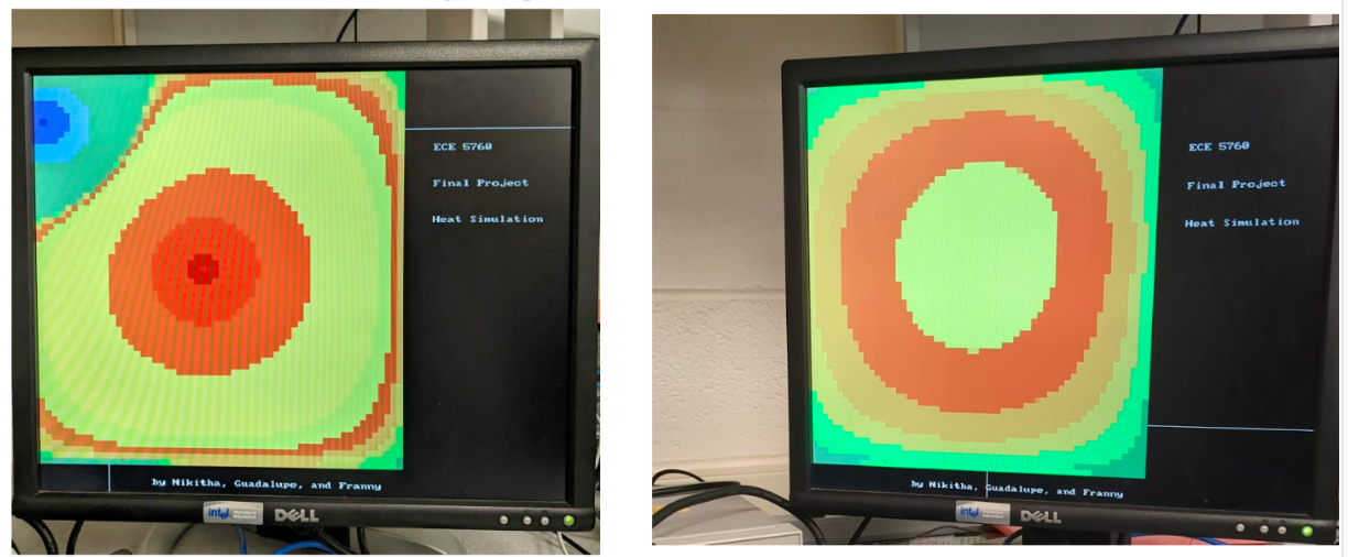
When trying to decide the scope of extra features we wanted to implement and create a plan for the high level design, we began by implementing the heat equation in C++ on our computers using GLUT through OpenGL. Once this was functional and we had a clear idea of how to incorporate sources, sinks, and initial heat to the discrete heat equation by initializing the cell values we moved the C code to the HPS, removed the graphics, and plotted directly to the VGA by plotting to every pixel in a square section and sending the color. The figures below show this result over time with three heat sources and one smaller heat sink.
HPS Design
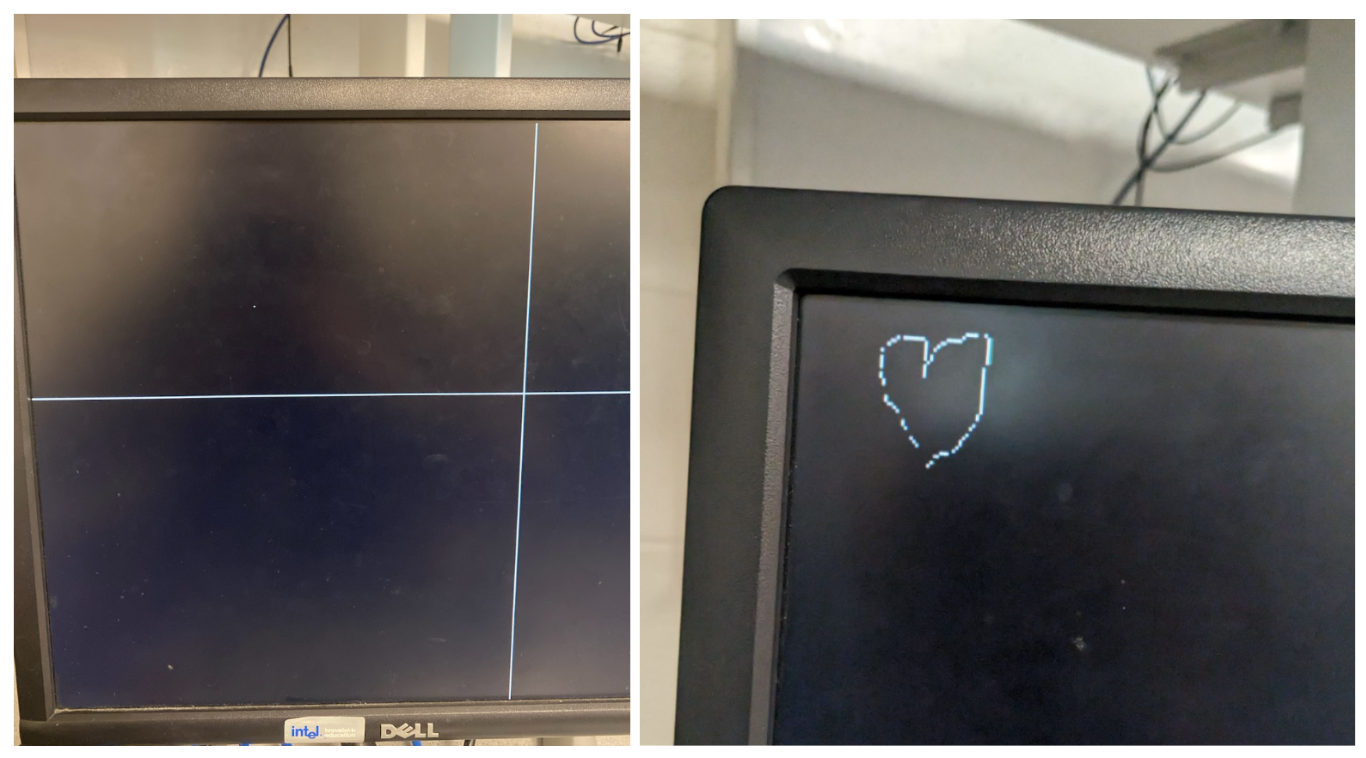
Doing this allowed us to incrementally implement the basic communication between the HPS and the FPGA. First we added a keyboard interface to the HPS code so that we would be able to select what type of heat we wanted to add. Then we added a cursor that would update live, and finally we implemented pixel by pixel drawing from the FPGA to the HPS as seen by the heart that we drew with the mouse that the HPS sent pixel by pixel to the FPGA.
With the ability to transmit pixel information directly to the FPGA we switched to integrating the ModelSim heat equation outlined in the section. But because of how we had implemented the pixel drawing, we quickly realized that we did not have enough M10K blacks to draw the whole screen. So instead we implemented a scaling system whose progress can be seen below. First we implemented a scaling system so that when the user clicks on the screen that position is scaled down by 7 and cropped to a square range of 64 by 64 possible positions. Then this information is transmitted to the HPS DPS Module, which simply receives the pixels and sends them to an arbiter to plot. This arbiter would then scale the 64 by 64 pixels back up to a square of size 448x448 pixels.
Modelsim Testing
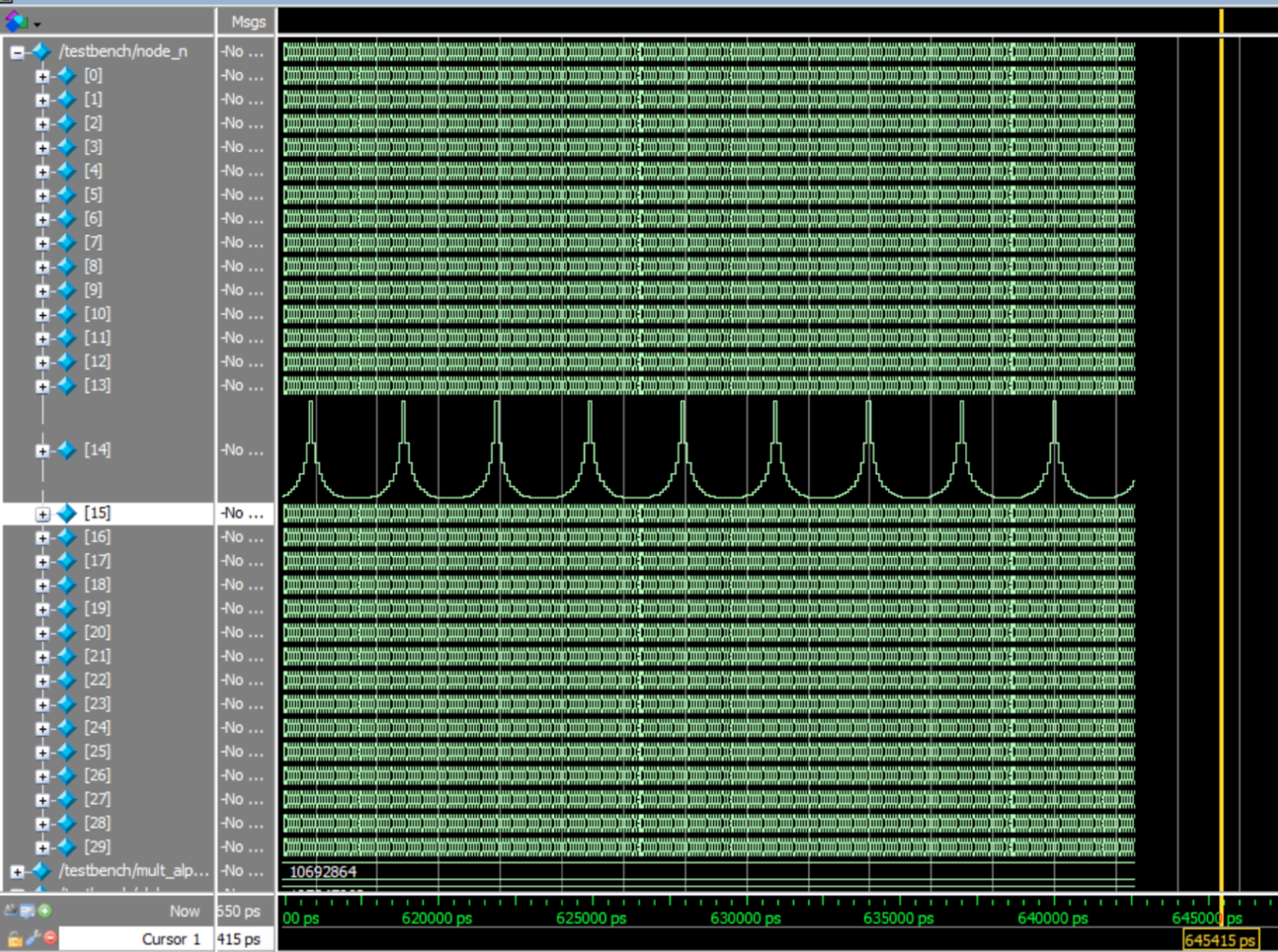
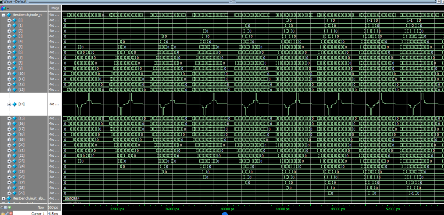
We tested the math/functioning of the heat equations on ModelSim before we began integrating it to run on the FPGA. We used a modular approach to our design and used 2 modules besides the testbench to implement the heat equations. We checked this system initially for a 30x30 grid, with a source being hardcoded in the center of the grid. The source value was set to a high value or decimal 8. We initialized all the other grids to have a value of 0. The compute module within our modelsim files was responsible for calculating the value of the nodes. The compute module does this by taking into account the neighboring grid values and using Alpha and delta constants, computing the new value for the grid being passed to this module. This module was instantiated within the column module, which was responsible for building one column. The column module has an M10K block to store the values of the columns. This also makes accessing the left and right values of the grid easier, which is needed to fully compute the grid values. In the testbench, we instantiate the 30 columns using the generate module and check the data of the center column to verify that the values are as expected and approximately the same value as the C++ implementation.
The results of this can be seen in the figures below. The node_n value is the value of each row in the column over one time step and then the next time step and so forth. We steep a steep increase, which is proof that the source is set and that as time passes by, the nodes closer to the source increase as well.
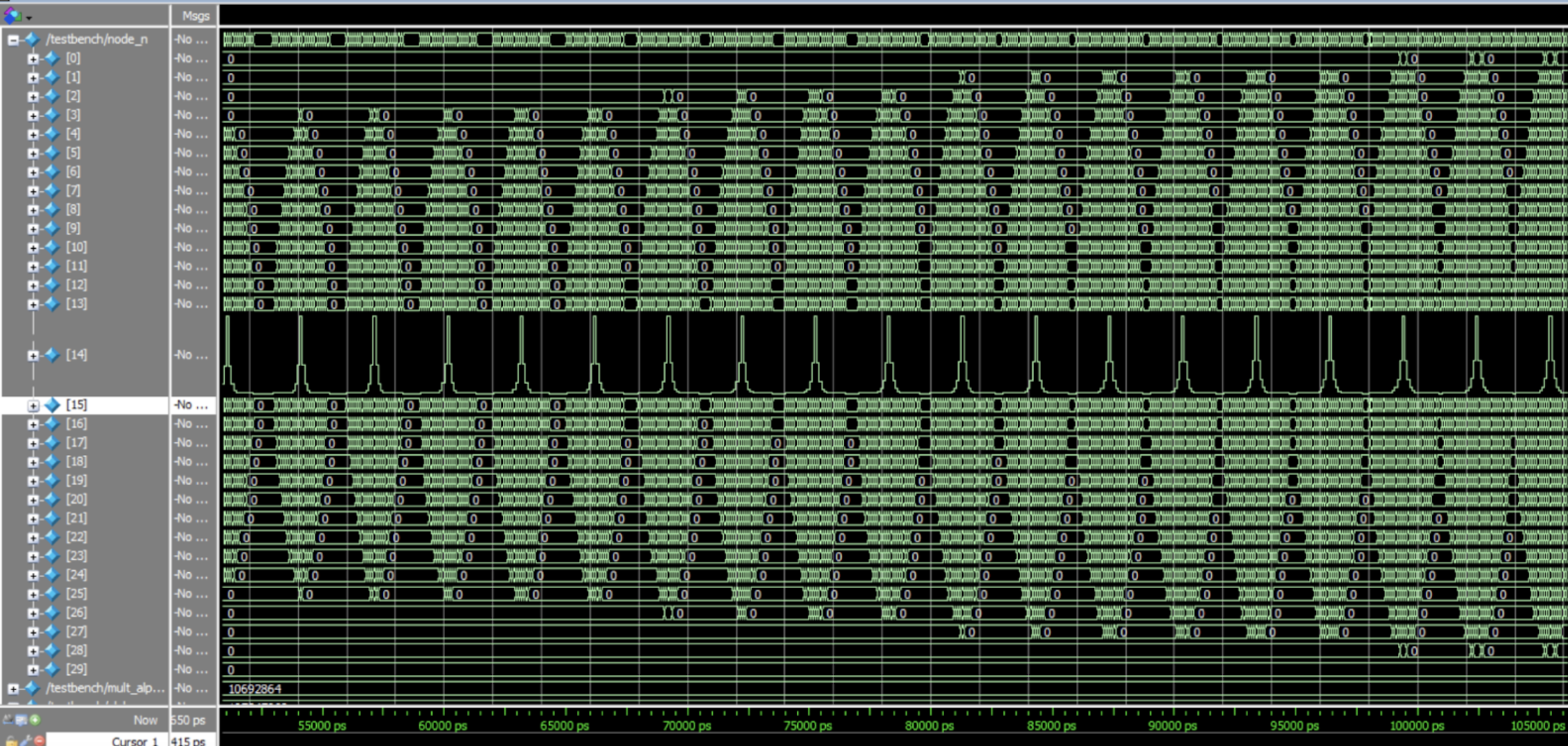
After we were sure that the source was working as expected, we added a sink in the same column. We hardcoded the sink at row 7 in the 15th column and when we observed the node values across this column, we saw that the waveform had a dip and a peak, which accurately represented the source and the sink. With this, we knew that our computations were accurate and it was time to run it on the FPGA.
FPGA Design
The HLD section goes over in detail the different modules included in the Verilog design. In this section we will go over details about what worked well and what didn’t along with details on the hardware. In our FPGA design for this project, we aimed to create a seamless and user-friendly interface for displaying and interacting with the heat simulation. Initially, our plan was to assign each pixel on the screen as a representation of one grid center. However, due to the limitation in the number of available M10K blocks, we had to adjust our approach. Instead, we decided to treat a 7x7 pixel area as one grid center. During the integration process of the ModelSim heat equation implementation with the plotting system connected to the HPS, we encountered several structural challenges. One significant issue was determining which modules had access to which M10K blocks. To address this, we implemented synchronization signals to ensure that the compute modules would only compute a single row and then wait until a signal was received before moving on to the next row. This allowed the higher-level modules enough time to send each computed value to the arbiter, which was responsible for plotting the results on the VGA screen. These adjustments and the introduction of synchronization signals helped us overcome the structural issues and successfully integrate the different components of the system.
Results
The speed of execution is incredibly fast and can be used live without any visible delay by users. The parallelization using the M10K blocks worked incredibly well for calculating the heat equation and the use of the GPU to plot through the SRAM also assisted in our ability to display live every time step iteration. We verified the correctness of our implementation by checking the point values in the first few timesteps manually. This was the same method of verification that we used to debug our modelsim implementation as well.
The user interface is incredibly user-friendly and easy to use as we ended up having to scale down some of our initial plans for HPS control. The user only has to run the executable file on the HPS and then can begin clicking wherever on the screen they would like to inject heat. Future progress can definitely be added here, our next step that we actually had implemented was giving the user the ability to differentiate between injecting heat and removing it using left and right button clicks, but unfortunately ran out of time for this addition on the FPGA side. The addition of sources and sinks is not as user friendly as this is currently hard-coded into the Verilog implementation.
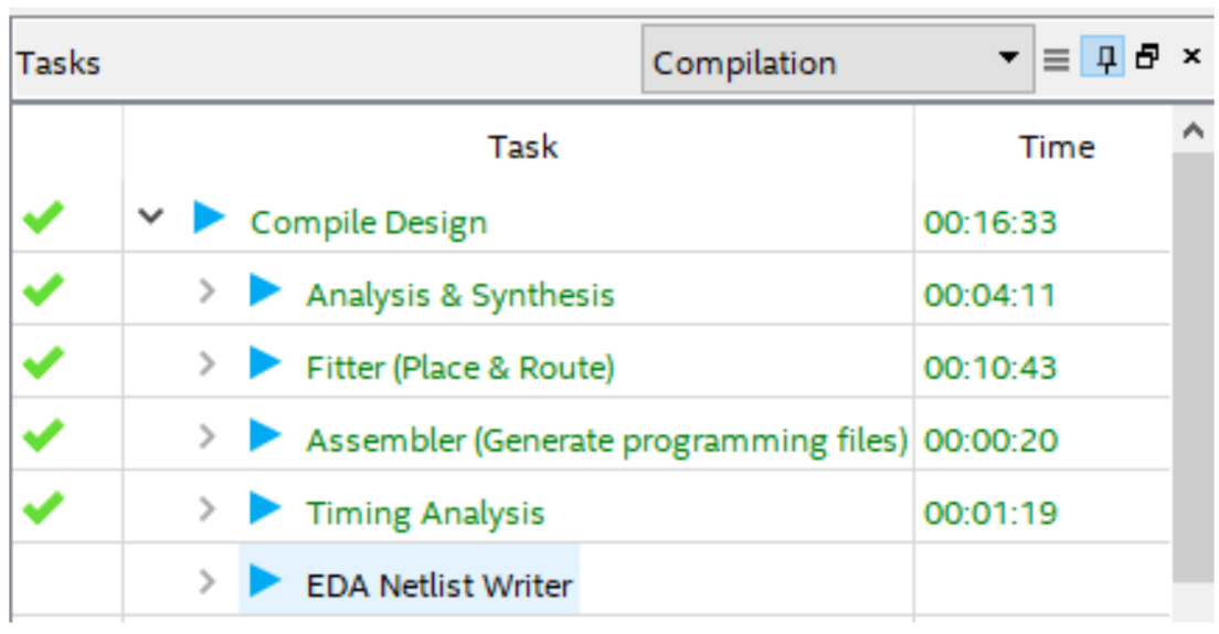
Compile Time
The compilation took about 16 minutes to run each time and this caused issues when we wanted to modify signal tap parameters. Everytime we made a change to the code and wanted to test it, we would have to compile it and then recompile it with the modified signal tap signals. Another issue we faced was that since we were using a lot of M10K blocks in our design too, we were limited by how many memory blocks we could use for signal tap. This really pushed us to understand our code better and debug smarter by picking the signals we needed for debugging only.
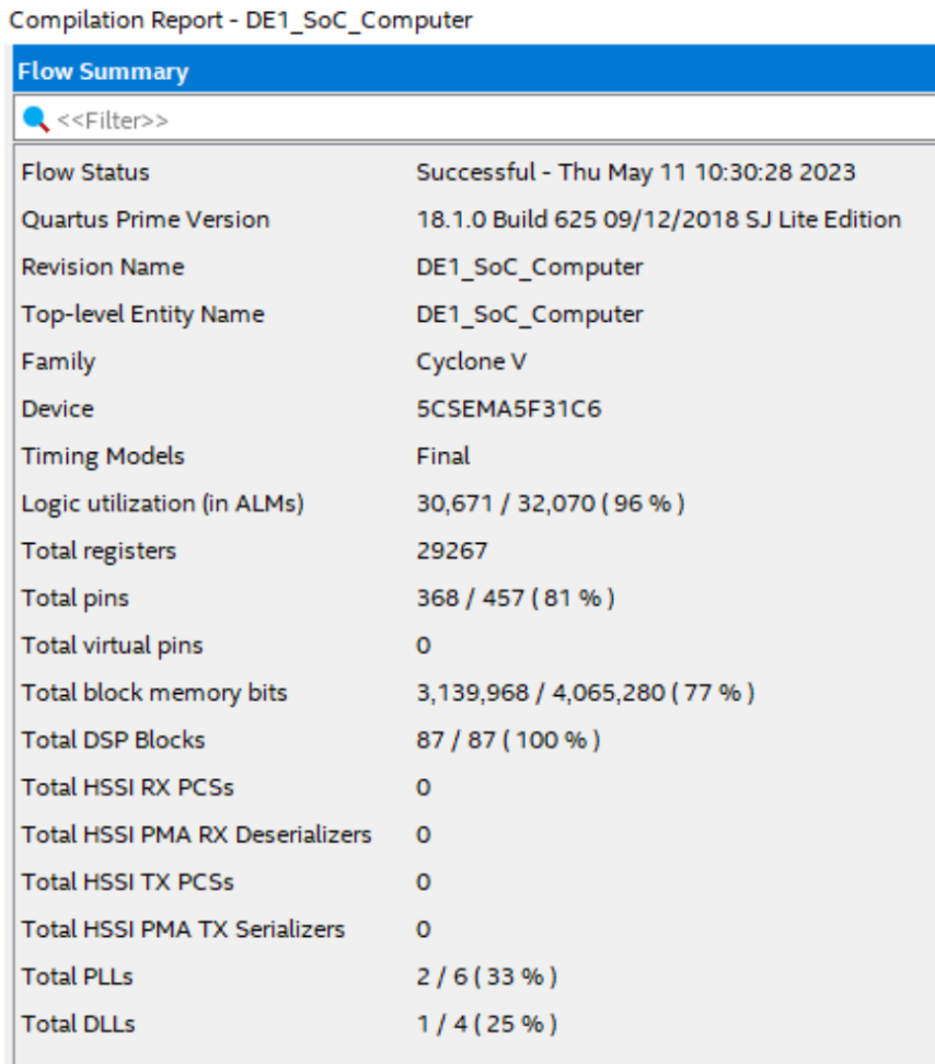
FPGA Resources Used
Conclusion
In conclusion, we successfully created an interactive heat diffusion simulation using the discrete heat equation that allows users to inject heat into a plane and see the results on the VGA screen directly. We have two compiled FPGA designs that can be programmed onto the hardware, one option has just a blank screen for a user to draw on and the other one has a source and a sink, but still allows the user to inject more heat and observe how the heat flows.
While we initially planned to have the user be able to control more of the design, we did not realize how quickly the project would scale up in size on the Verilog side and had to scale down our goals. In spite of this, we are very proud of how the project turned out. If we were to do this again we would spend a lot more time planning out how all of the Verilog modules would interact with each other early on, as this might have led to us coming up with solutions to structural issues faster. We were very careful about pushing every version and small progress made to github and this allowed us to successfully backtrack multiple times and is something we would most definitely do again. We did use the GPU with FAST display from SRAM sample code that was provided and used in the class, but aside from that we did not use any other external materials. Even the color scale we made ourselves!
Check out the video below to see our project!
Appendix A (permissions)
The group approves this report for inclusion on the course website.
The group approves the video for inclusion on the course youtube channel.
Fully commented Verilog, C, and testing code can be found at the following link: https://github.com/fran07981/ece5760finalproject
We used extensively the documentation provided on the course webstie linked here: https://people.ece.cornell.edu/land/courses/ece5760/
Hunter's Drum Slides: https://vanhunteradams.com/DE1/Drum/Drum.pdf
All members participated in debugging, integration, and documentation.
Guadalupe wrote the initial C implementation and defined and implemented the communication of data between the HPS and the FPGA.
Nikitha implemented the Modelsim implementation of the discrete heat equation and testing.
Franny worked on the HPS code to read information from the mouse and keyboard and plotting the cursor as well as Verilog debugging and making the color pallet.