Jichao Yang (jy874), Yiyang Zhao (yz2952), and Ang Chen (ac2839)
Demonstration Video
1. Introduction
Handwritten digit recognition could be achieved through a custom hardware implementation of Convolutional Neural Networks (CNNs) in Verilog, enhancing efficiency and speed for real-time applications.
In this project, we endeavored to accelerate handwritten digit recognition by leveraging the power of Convolutional Neural Networks (CNNs) and implementing the entire architecture in FPGA.
We started by coding each layer of the network in Verilog and rigorously testing them in ModelSim. After ensuring the timing was correct, we used Python scripts to validate their functionality. Then, we integrated these layers into a cohesive system and built a data flow mechanism from the user image through all these layers to the output. In addition, we trained a CNN model using PyTorch on the MNIST dataset and extracted the weights for both the convolutional and fully connected layers. These weights were loaded into our hardware system, priming it for recognition tasks. We extensively tested the system's accuracy using both MNIST dataset digits and real handwritten samples.
By moving computation from software to specialized hardware, we aimed to significantly boost performance and efficiency, enabling rapid and accurate recognition of digits.
2. High Level Design
2.1 Background Math
In this section, we discuss the fundamental mathematical concepts that underpin the architecture of Convolutional Neural Networks (CNNs). These concepts include convolution, pooling, ReLU activation, and fully connected layers.
a. Convolution
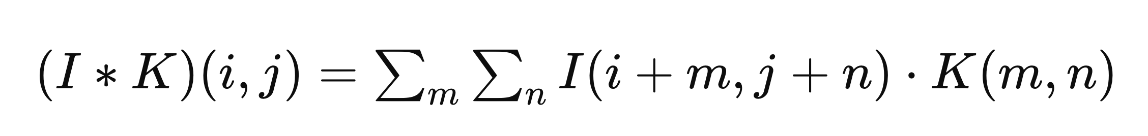
Convolution is a mathematical operation used to extract features from input images. It involves sliding a filter (or kernel) across the input image and performing element-wise multiplications followed by summations. The result is a feature map that highlights the presence of specific patterns in the image. Mathematically, if 𝐼 is the input image and 𝐾 is the kernel, the convolution operation 𝐼 ∗ 𝐾 at a position ( 𝑖 , 𝑗 ) is given by:
b. Pooling
Pooling is a down-sampling operation that reduces the dimensionality of feature maps while retaining important features. The most common type of pooling is max-pooling, which selects the maximum value from a region of the feature map. This operation reduces computational complexity and helps in achieving spatial invariance. For example, a 2x2 max-pooling operation on a feature map selects the maximum value from each 2x2 region.
c. ReLU Activation
ReLU (Rectified Linear Unit) is an activation function used to introduce non-linearity into the model. It is defined as:
This function sets all negative values in the feature map to zero, allowing the network to learn complex patterns. ReLU activation accelerates convergence and mitigates the vanishing gradient problem.
d. Fully Connected Layers
Fully connected (FC) layers are used at the end of the CNN architecture to perform classification. Each neuron in an FC layer is connected to every neuron in the previous layer. The outputs from the previous layers are flattened into a single vector and multiplied by a weight matrix, followed by the addition of a bias term. This process is described mathematically as:
where 𝑥 is the input vector, 𝑊 is the weight matrix, 𝑏 is the bias vector, and 𝑦 is the output vector. The final layer uses a softmax function to convert the outputs into probabilities for each class.
e. Mathematical Representation
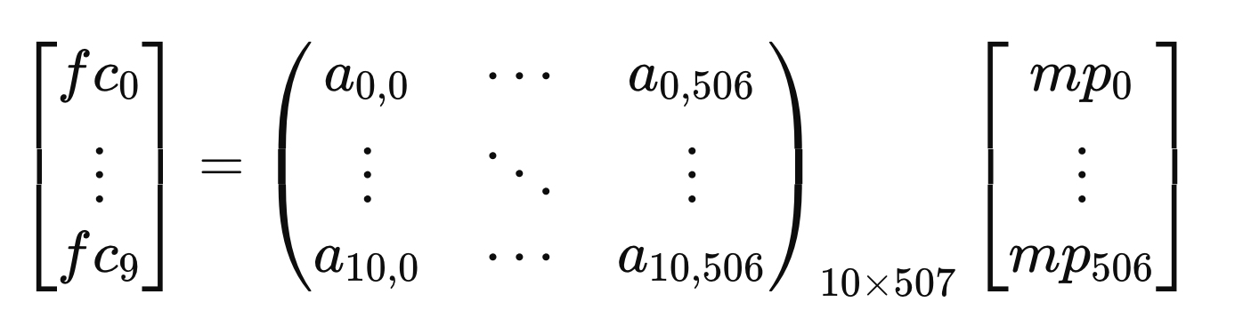
The output of the fully connected layer, denoted as 𝑓𝑐 , can be represented as follows:
where 𝑓𝑐 is the output of the fully connected layer, mp is the output of the max-pooling layer, and the 10 × 507 matrix is the weight matrix.
These mathematical principles form the foundation of the CNN used in our hardware implementation for handwritten digit recognition. By understanding these concepts, we can effectively design and optimize each layer of the network to achieve high accuracy and performance.
2.2 Logical Structure
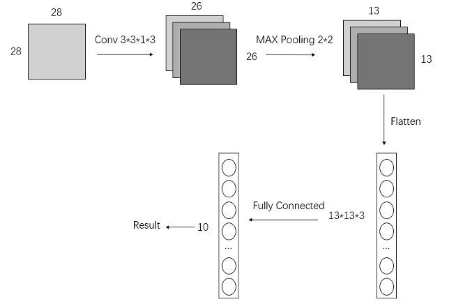
We proposed a CNN architecture for this multi-classification task, which includes a convolutional layer, ReLU module, max-pooling layer, and fully connected layer. As illustrated in Figure 1, the input image is an 8-bit grayscale image with dimensions of 28x28 pixels. In the convolutional layer, we use three 3x3x1 kernels, as our input image has only one channel. There is no padding, and the stride length is 1. The output of the convolutional layer is a feature map with dimensions of 26x26x3, which is then passed through the ReLU module. The max-pooling layer has a kernel size of 2x2 and a stride length of 2, with no padding. After max-pooling, the resulting feature maps have dimensions of 13x13x3. In the fully connected layer, the 13x13x3 feature maps are first flattened and then multiplied by the corresponding weights, resulting in the final output.
Figure 1: CNN Structure for This Project
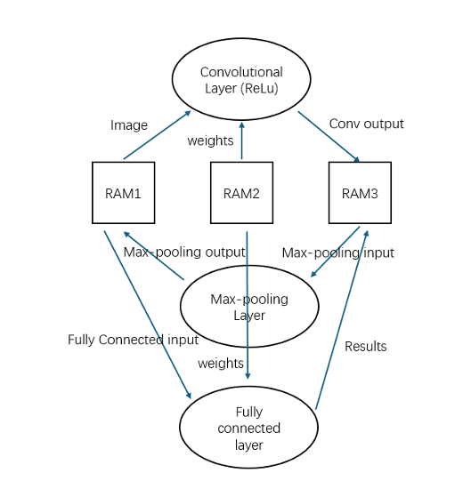
In our hardware design (Fig. 2), we integrate three neural network modules with three SRAM units. The SRAM units are crucial for data exchange, storage, and transmission. SRAM1 stores the image data, while SRAM2 holds the weight data for the convolutional and fully connected layers. SRAM3 stores the convolution results, which serve as input for the max-pooling layer. The output of the max-pooling layer is then stored in SRAM1, which becomes the input for the fully connected layer. The final results are stored in SRAM3. Multiplexing is necessary due to the dual utilization of SRAM1 and SRAM3 and the simultaneous read/write operations by the neural network module. Since SRAM2 stores weights for both layers, it also requires multiplexing for simultaneous access by two modules.
Figure 2: Data Flow between Each Layert
3. Program / Hardware Design
3.1 Hardware Design
a. Convolutional Layer
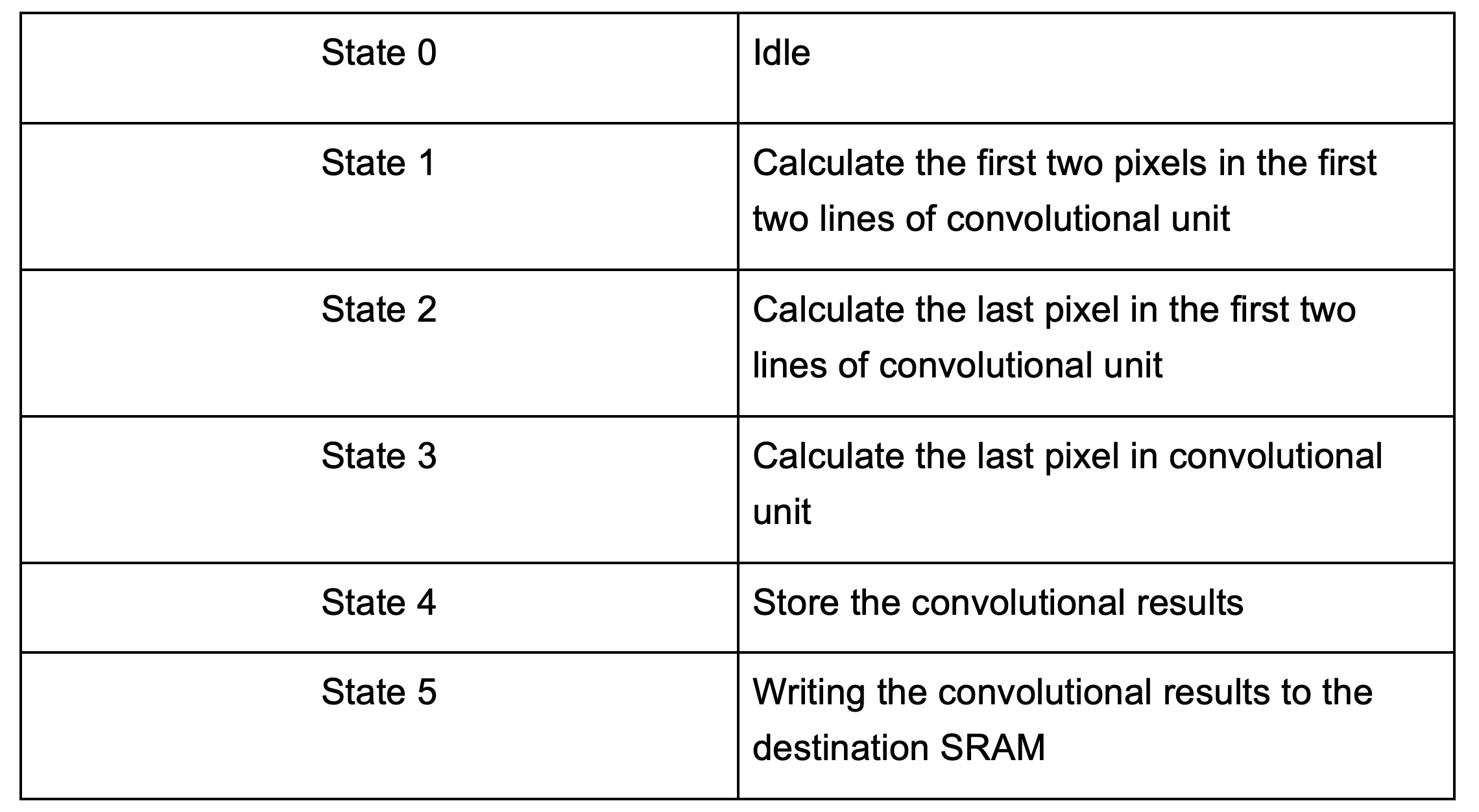
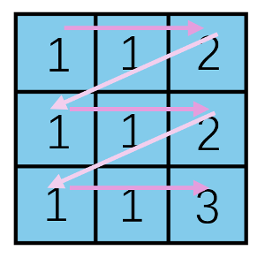
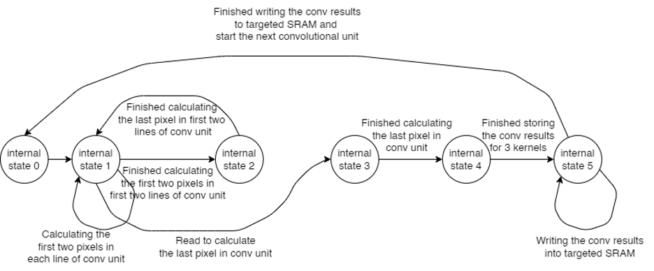
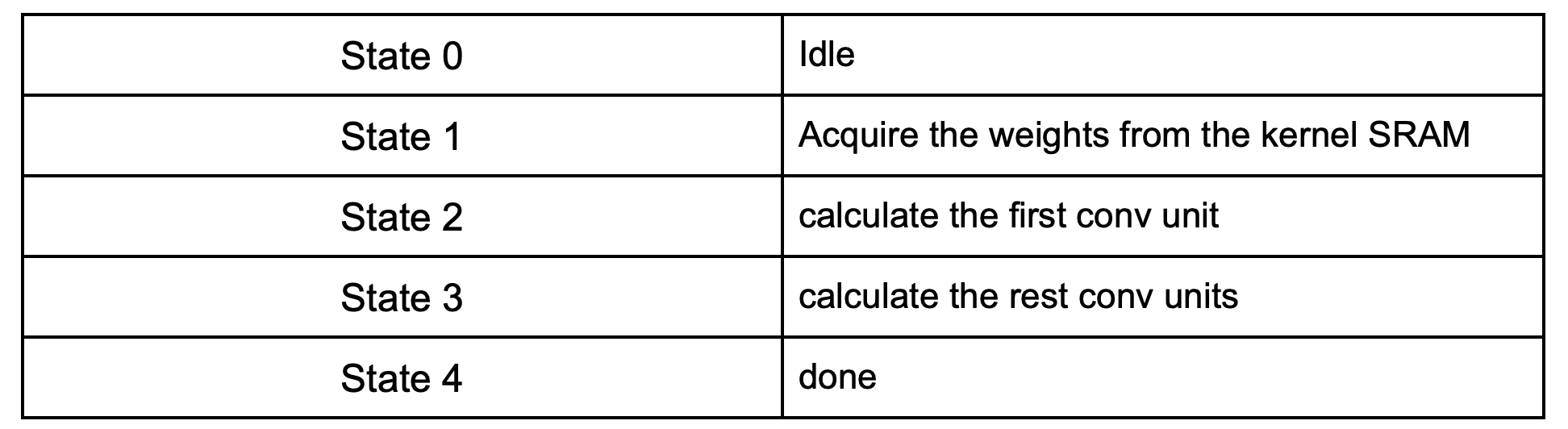
In our convolutional layer design, we use one multiplier for each convolutional unit, which is the minimum component required to perform the convolutional arithmetic. As illustrated in Fig. 3, at least nine clock cycles are needed to complete the convolutional operation. The process begins with the top-justify pixel in the kernel. In each subsequent cycle, the operation moves to the next pixel to the right, performs the multiplication, and accumulates the result with the previous value. This process repeats until the entire convolutional unit is calculated and the accumulated value is output. A state machine controls this process (Fig. 4). The table below shows the action for each state, and the numbers in Fig. 3 indicate the current state for each pixel. Considering the idle state and data storage, 14 clock cycles are required to complete a convolutional calculation, as each result must be stored in the SRAM individually.
Table 1: Detailed Information for Convolutional Unit State Machine
Figure 3: Convolutional Unit
Figure 4: State Machine Transmission for Convolutional Unit
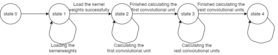
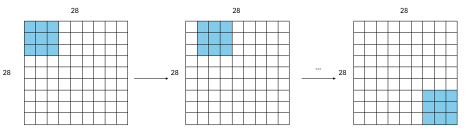
In the convolutional layer, we perform the convolutional arithmetic starting from the top-justify corner of the image. After completing one unit of convolutional arithmetic, the convolutional kernel moves to the next 3x3 area in the image to perform the next operation. This process repeats until the kernel reaches the bottom-right corner of the image. At this point, the outputs from the convolutional layer are stored in the designated SRAM, as shown in Fig. 6. We set up three parallel channels for this process. A state machine controls the operations within the convolutional layers. Fig. 5 illustrates the state machine transitions, and Table 2 details the actions performed in each state.
Figure 5: State Machine Transmission for Convolutional layer
Figure 6: Arithmetic Process of Convolutional Layer
Table 2: Detailed Information for Convolutional Layer State Machine
b. Max-Pooling Layer
In our design of the max-pooling layer module, we mirrored the control flow of the convolutional layer. However, the internal state machine is simpler, as the maximization operation requires less complex logic. In the IDLE state, the module waits for a commencement signal, which is also the end signal from the convolutional layer. Upon receiving this signal, it transitions to the CALC state. In this state, it traverses the input matrix to find the maximum value in each 2x2 subregion. Subsequently, it transitions to the WRITE state, where the maximum value is stored in the designated SRAM address. Finally, it reaches the DONE state, preparing for the processing of the next subregion.
c. Fully Connected Layer
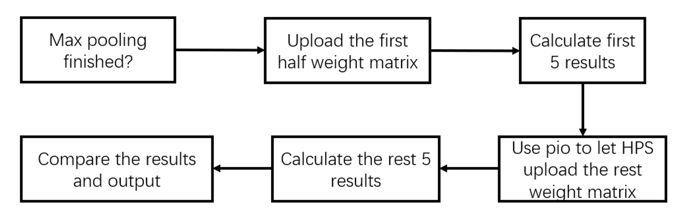
The fully connected layer converts the 507 outputs from the max pooling layer into ten output values. The highest output value is the recognized number. As the weight matrix has a size of 507*507, it is not possible to upload the matrix to SRAM at one time. Our solution is to upload the matrix and calculate the output two times. The final recognized number of the CNN will be shown in the digital display.
The fully connected layer involves 5 procedures:
1. Upload the first upper half weight matrix to the SRAM
2. Calculate the first 5 results
3. Tell the HPS to upload the rest fully connected layer matrix to the SRAM
4. Calculate the rest 5 results
5. Find out the highest value as the output recognized number
Figure 7: Computation Flow for fully connected layer
3.2 Software Design
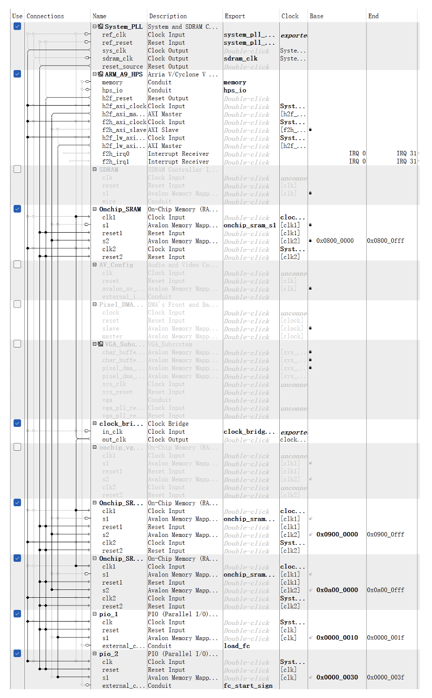
The HPS design is mainly about how to load the image, convolution weight matrix and the fully connected weight matrix to the three SRAM without exceeding the SRAM storage capacity. We set two pio ports for controlling the loading progress.
‘load_fc’ is an ‘input’ to the HPS, indicating that the max pooling process is finished. ‘fc_start_sign’ is an ‘output’ to the HPS. It allows the fully connected layer to start computation after loading all the weight matrix data.
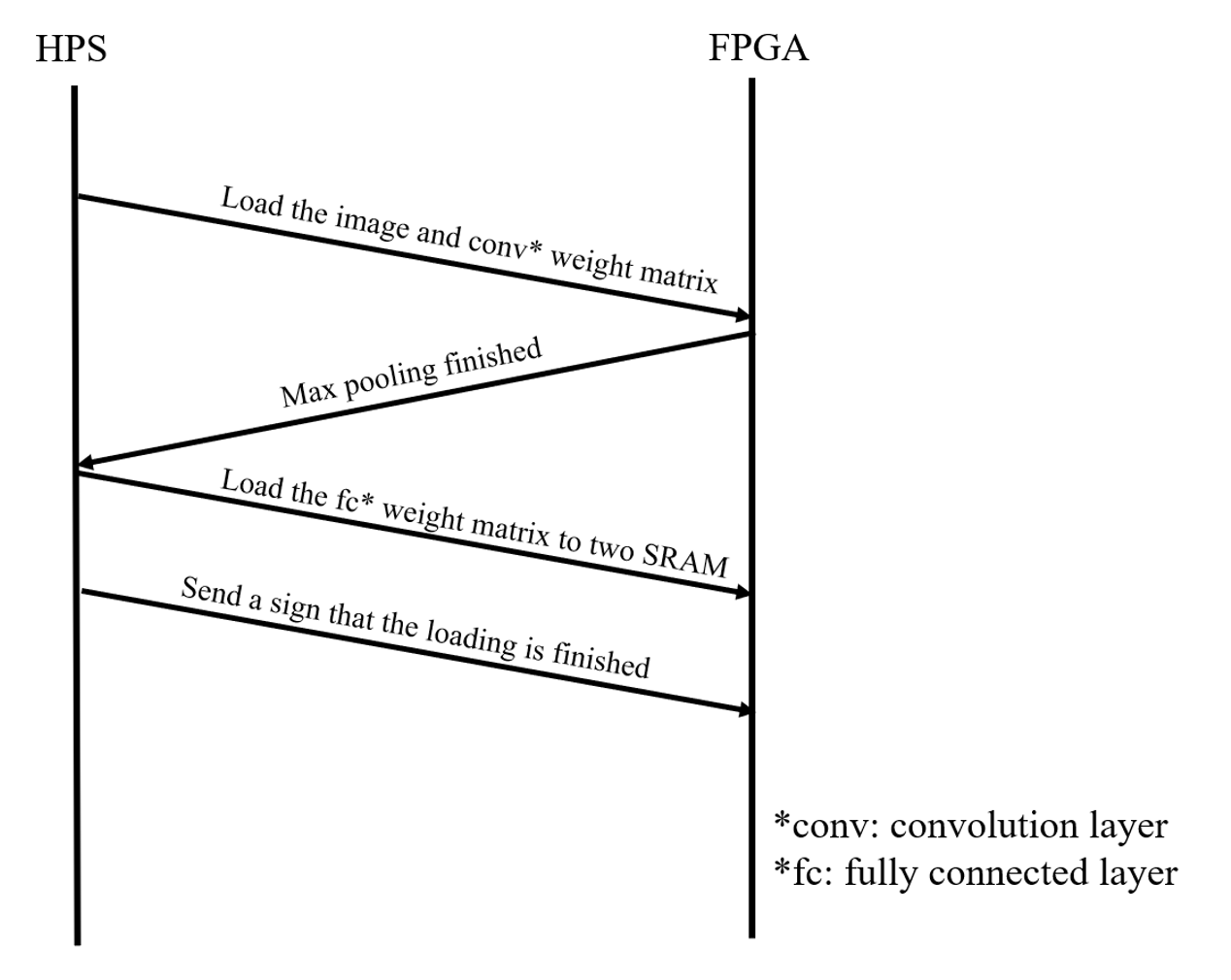
Initially, the process begins with the HPS loading the image and the convolution layer weight matrix into the SRAM. After the max pooling operation is completed on the FPGA, the HPS loads the fully connected (fc) weight matrix into two separate SRAMs within the FPGA. Once the fully connected weight matrix is loaded, the FPGA sends a signal back to the HPS indicating that the loading is complete. This sequence ensures that the FPGA has all the necessary data to perform the neural network computations. The process is illustrated in Fig. 8.
Figure 8: HPS-FPGA Communication Sequence for Neural Network Computation
Figure 9: Quartus Prime FPGA Component Configuration
Results
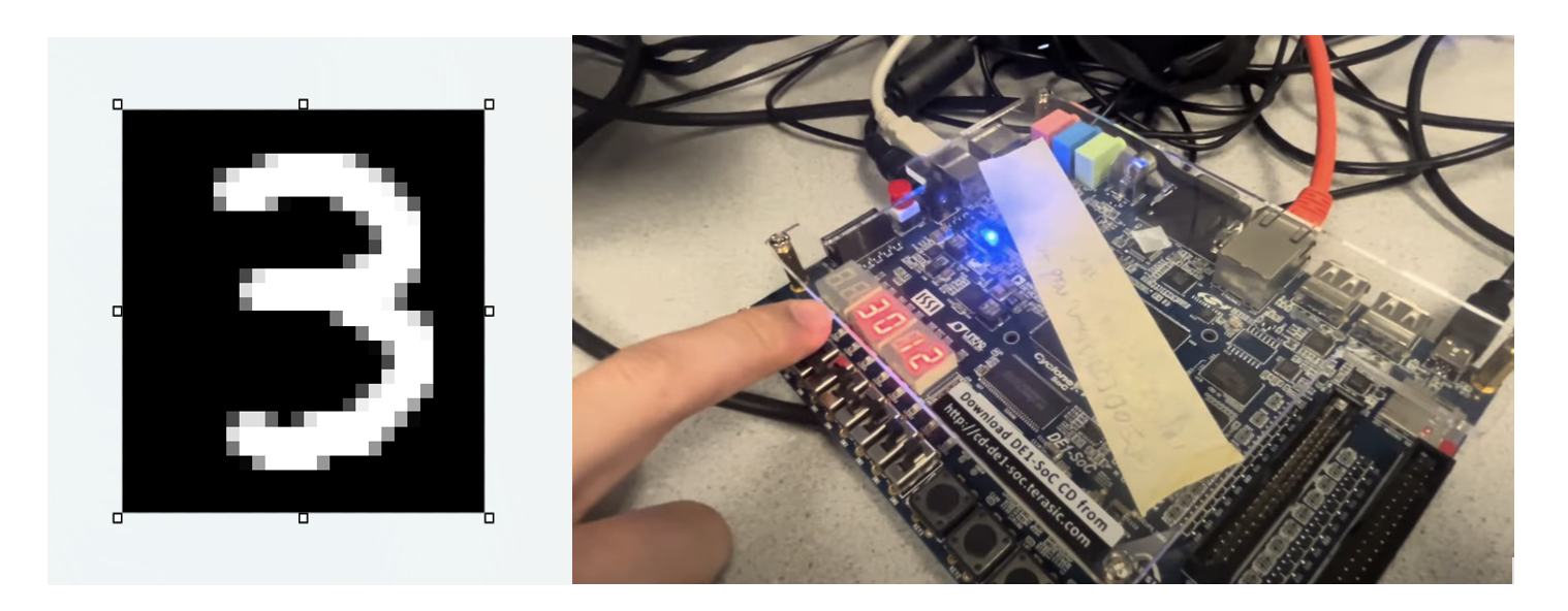
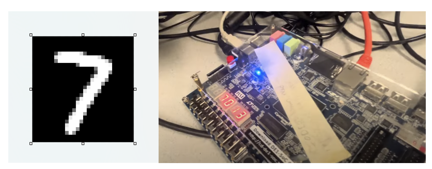
Some of the results are shown in the Youtube video demo. The highest bit represents the output:
Figure 10: Test Result for Number 3
Figure 11: Test Result for Number 7
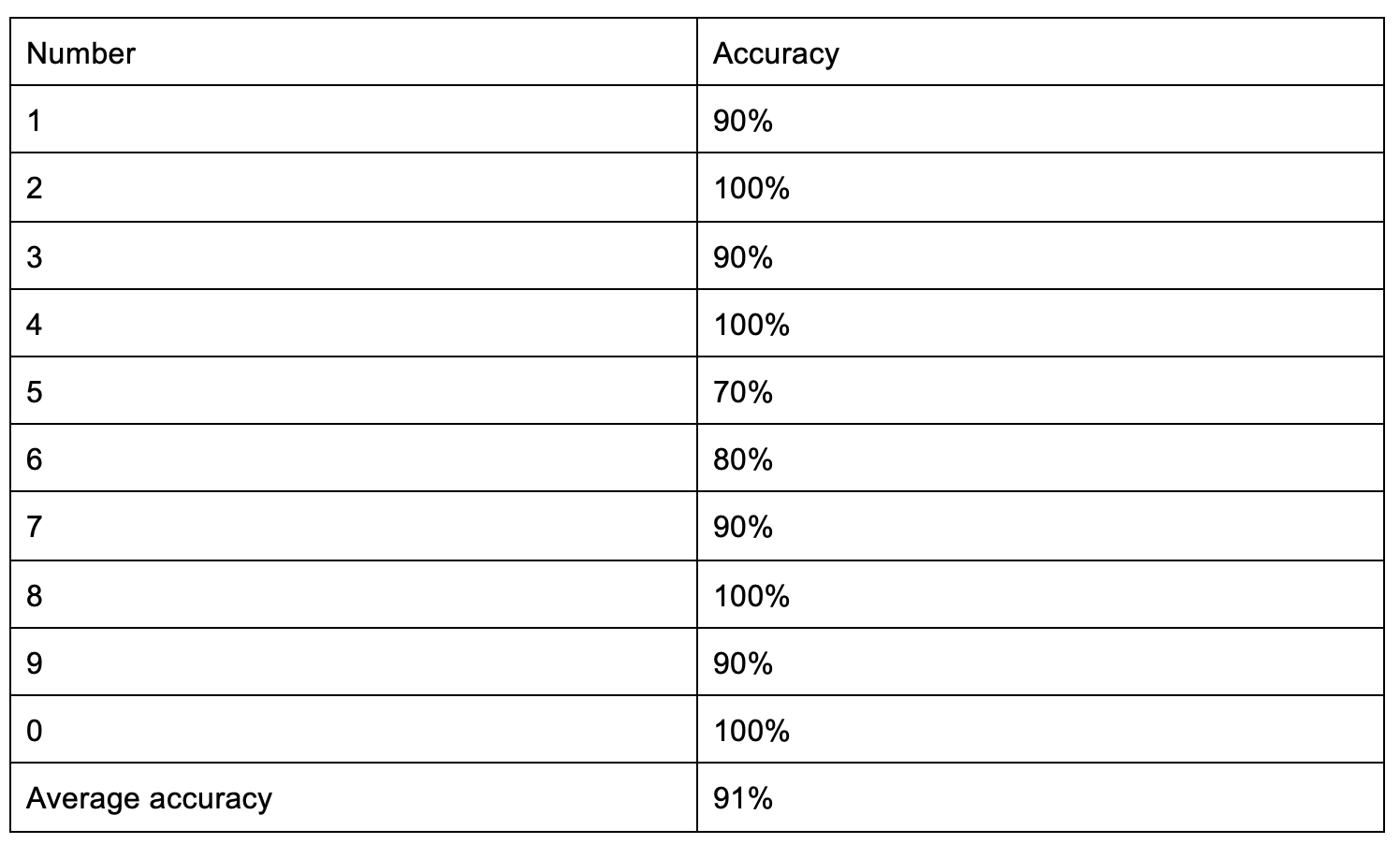
Table 3. FPGA Accuracy for Recognition, Each Number Tested 10 Times
Conclusions
Our design accelerates the calculation process of the CNN recognition algorithm. The average accuracy for our CNN on FPGA reaches to 91%. Further improvements can be done by adding a real-time camera, changing the fixing point to floating point and training a more sophisticated model in Pytorch to get a better weight matrix.
The code is our original program. Also, the design can be more complicated if we add more layers between the input and output.
Appendix
1. Permission
The group approves this report for inclusion on the course website.
The group approves the video for inclusion on the course youtube channel.
2. Code
The code we used to build our project is available at Digit Recognition