OPTIMIZATION OF AN
INTEGRATE-AND-FIRE NETWORK
TO SIMULATE
THE BEHAVIOR OF A CRICKET

More and more is understood about the nervous system of humans and animals. And once one understands the basics of it, one of the next steps is to build models and simulations for it, to be able to do more controlled and thorough testing.
However, the nervous system is very complex, and to build a realistic model of a nervous system of almost any animal, let alone humans, is a very difficult problem. The system is very high-dimensional, so that even when the composition of the system would be understood, the configuration of the parameters and different influential factors is still a non-trivial matter.

As a first step in learning about the behavior of neural networks and optimization over a large parameter space in such a network, we decided to start from the simulation of a known system. By using a system that already has been studied and used, we have the possibility of comparing our self-developed results to the previously published data. Thus we are able to make estimates of the accuracy and correctness of our way of simulating and optimizing.

In this project, we started from a simple four-neuron network to simulate the response of a cricket to input-sounds. The model was taken from the paper "A simple latency-dependent spiking-neuron model of cricket phonotaxis" by B. Webb ([2]). We took that network-configuration, and wrote our own programs to implement it in Matlab, using integrate-and-fire neurons.
First we compared different implementation methods on those neurons, comparing efficiency, correctness, etc. Then we used the chosen neuron-implementations to compose the complete network, and started working on a higher level.
Next we needed a measure, a standard, to compare results from different crickets. Once we decided on that, after testing several evaluation-methods, we were able to begin with the actual optimization of our cricket-model.
This led to another difficult decision, as to which optimization algorithm to use. There exists a large number of different optimization procedures, all of which have there own advantages and disadvantages. In the end, we chose to use a genetic algorithm for optimization, because of the ease of implementation, and because tests had shown that the performance was good enough for our purposes in this project.
Finally, using the genetic algorithm, and varying the level of complexity of the parameter set, we were able to find some range of optimal crickets, and to derive conclusions about the possibilities and limitations of this simplified model.
We also wanted to see if it was possible, using this simplified system, to create different "species" of crickets. We defined these different species by a feature that is known to differ among different species of crickets in nature: we changed the time-interval between consecutive bursts of input-sounds. Thus each species of cricket is supposed to recognize its own typical sound.

Finally, we started working with a biologically more correct network, using 6 neurons, and tried to get the same kind of results, by doing optimization through the same algorithms and programs.

The basic outline of the network we used for our experiments was based on the article "A simple latency-dependent spiking-neuron model of cricket phonotaxis" by B. Webb and T. Scutt ([2]).

It is a simplified network consisting of 4 neurons (see Fig.1).
2 ascending neurons, AN1 neurons, left and right (ANL and ANR), receive auditory input from left and right ear respectively. Each of these AN1's has an excitatory connection to an ipsilateral motor neuron (MN), and an inhibitory connection to a contralateral MN. These MN's send output to the muscles that control the body motion.
Because of the configuration, if both AN1's are equal in their parameters, a MN will typically have an increase in its potential when the ipsilateral AN1 neuron starts firing before the contralateral AN1 does.

Fig.1 Experimental neural network: 2 Ascending Neurons of type AN1, left and right (ANL and ANR) have connections with excitatory synapses to the ipsilateral Motor Neurons (MN's) and with inhibitory synapses to the contralateral Motor Neurons.

The parameters of this network were determined experimentally, to generate an optimal network.

Faze 2

In the second faze, we wanted our model to be more biologically correct. In reality, the inhibition of movement of one side of the body does not happen through inhibition of the AN1's to the contralateral MN's. Instead, there is a third type of neuron involved, the Omega Neurons (ON1). They are called this way, because of their shapes, that resemble the Greek capital Omega-letter. There is one ON1 on each side of the body (in the head).
These ON1's receive the same auditory excitatory input as the AN1's, directly from the ipsilateral ear. When spiking, an ON1 inhibits both the contralateral AN1 and the contralateral ON1.

Fig.2 Biologically more correct neural network: 2 Ascending Neurons of type AN1, left and right (AN1L and AN1R), have connections with excitatory synapses to the ipsilateral Motor Neurons (MN's). 2 Omega Neurons of type ON1, left and right (ON1L and ON1R), get the same input as the AN1's, and have connections with inhibitory synapses to the contralateral AN1 and the contralateral ON1.

Experimental setup

All experiments were done mathematically, by simulations, using Matlab. To get some kind of visual form of comparison, we built a simple and small system: we placed a sound-source at a certain position in a 2D plane, put a simulated cricket in a different position, and made the cricket move according to the output of the simulated nervous system, the output of the MN's.

In Fig.3 you can see the test-plane: the sound source is indicated by a small cross, the cricket is represented by 3 circles: it's body, enclosed between its 2 ears. These ears are so big, to show the time-delay between the sounds, received in both ears. This sound delay is significant enough to be detected by our network, simply by comparing and working with the spike trains, although by eye one hardly sees the difference.
The default behavior of the cricket is to move straight forward; our neural network tells it when to turn. And because the sound source isn't right in front of the cricket, the sound-delay in both ears will cause the system to indicate necessary turns.

Fig.3 View of the test-plane. The small 'x' indicates the position of the sound source, the cricket is represented by 3 connected small circles: its body and ears.

Optimization methods

Faze 1

First we wanted to test the influence of the synaptic weights on the cricket's behavior (the system's output). This had the big advantage that the searches only happened over two free parameters, i.e. in 2D-space, and thus the results could be plotted out as a surface. This enabled us to get some visual idea of the results.

After building a relatively successful cricket, we still needed to optimize the rest of its parameters, to find an optimal cricket, and maybe find the key between different "species" of crickets.
We already had some general idea of realistic and good value-ranges for some of the parameters, but we wanted to be able to localize an optimum in a greater parameter space. Therefore we tried to find that optimum by using the "fminsearch"-function in Matlab. But because of the nature of the surface (a lot of flat  plateaus), this function did not give the results we hoped for. The optimal values that were returned, were mostly very local, and thus extremely dependent on the initial point.
So we turned to another method: we started optimizing by implementing a genetic algorithm, based on the chapter "Optimization of swimming locomotion by genetic algorithm" by D.Barrett in the book "Neurotechnology for biometric robots" ([5]).

The algorithm works as follows:
You start by building the "definition" of an instance of the object that has to be optimized, i.e. listing all parameters that are to be optimized by the genetic algorithm. Then you have to choose the ranges of values for each of the parameters. These decisions are up to the programmer, and can influence the outcome and performance of the algorithm significantly.
The algorithm then starts with one generation, consisting of a certain number of species (i.e. parameter sets). The values of each of these parameters in each of the animals is chosen at random from the ranges for the respective parameters. Then the program evaluates each of these animals and keeps only half of them: those that gave best results.
After this the actual genetic part of the algorithm takes place:

• Reproduction: the remaining animals are doubled, such that we have again the full number of parameter sets.
  
• Crossover: divide the parameter sets in pairs, and for each pair of animals, a certain place in the list of parameters is chosen at random, and all parameter values after that place are switched between both crickets. This is the kind of crossover as it happens with chromosomes at the duplication of a cell.
  
• Mutation: by a fixed (low) probability, one parameter in the whole generation gets a random new value. This probability must be determined by the programmer, but is typically dependent of the number of animals per generation and the number of parameters per animal.

We also considered the use of a variant of simulated annealing, but we decided not to, for several reasons. The most important reason was the ease of programming and the understandability of the program. This system was intended to get an idea of the general principles of such a system, of what the possibilities are, how far we could drive it, etc. The genetic algorithm seemed to work well, and was relatively easy to program and to understand. Simulated annealing would increase the complexity of the program, while probably not increasing the performance terribly much.

From all crickets that came out of different runs of the genetic algorithm, we extracted the best one, by testing each "converged cricket" on the same big number of different sound source positions. The best cricket was the one reaching the most sound sources and defined to be "species A".
After that, we did the whole optimization process over again, to create "new species". We defined these new species by changing the interval between different bursts of input sounds in the optimization process. This is a feature, known to differ between different species of crickets in nature.

After creating different species like that, we wanted to compare them in parameters and in performance, to see if there were certain parameters that were significantly different. These would then determine to which inter-burst-interval a certain species of cricket would respond.

Faze 2

With the biologically more correct system, we basically ran the same tests, used the same algorithms. Again we wanted to find the optimal parameter setting for the cricket-simulation. Because of the generic nature of the code, it was fairly easy to adapt the code to the slightly more complex system.

From the plots and data from [7], it was clear that the ON1's had practically the same parameter values as the AN1's: time constants, threshold, resting potential... All seemed to be very similar or equal. So that gave us a lot of tight constraints on the new neurons, even before any of the optimizations.

---

3. RESULTS

Different comparison measures

To test and compare the different parameter settings of the cricket, we tried different evaluation schemes. In all tests we let the cricket move for a limited period of time, approximately equal to twice the time it would need if it would move in a straight line towards the sound source. At the same time we tested the influence of the synaptic weights on the cricket's performance. Because this is a 2D-search, we could plot out the results of all crickets as one big surface, and have a visual image of the results. This also simplifies the comparison of the different comparison measures.

First we computed the minimal distance that is created between the sound source and the middle of the cricket's body, at any point of the cricket's path through the plane. (Fig.4a)
Secondly, we recorded the time needed by the cricket to get within a certain very small range of the sound source. If the cricket never got there, the end-time of the interval was returned. (Fig.4b)
Finally we measured the "angular delay" of the cricket's path to the sound source. To do this, at each point in time, we computed the difference in angle between the cricket's current orientation and the angle of the straight line from its position to the sound source. The absolute value of this angle-difference was added to our comparative measure. The total sum of the angles, until the cricket gets within a certain small range of the sound source, forms the resulting value. (Fig.4c)

We applied each of the performance-measures to a large number of different crickets, using as parameters a wide range of values for the 2 synaptic weights. We chose the synaptic weights to be symmetric and non-variable. So both excitatory had the same weight, as did both inhibitory synapses, at all times during a run of the program. (See Fig.4)

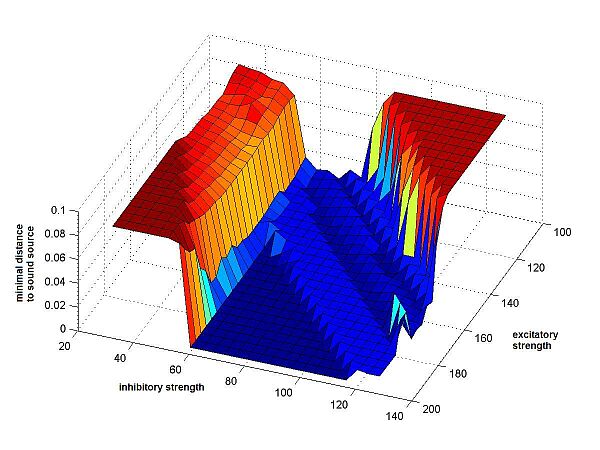Fig.4a Minimal distance from sound source

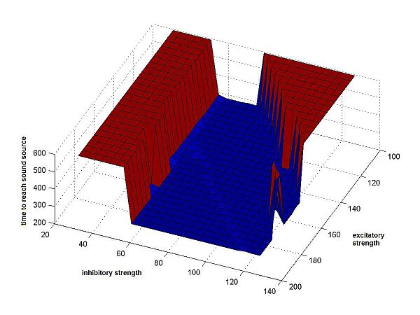Fig.4b Time to sound source

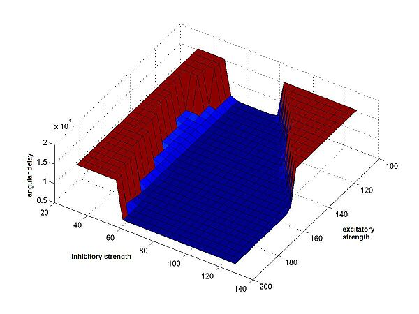Fig.4c Angular delay along path

Fig.4 Resulting surfaces for the 3 different performance measures. On the axes, the synaptic weights have been multiplied by 10. The values of the excitatory synapses range from 10 to 20, the values of the inhibitory synapses from 3 to 13. Along the z-axis the results are shown, as returned by the cricket-function, results that have different meanings on each plot: 3a The result is the minimal distance between cricket and sound source, at any point along the path of the cricket. 3b The result is the time it took the cricket to get within a small area around the sound source. If this area is never reached, the end of the time interval (600) is returned. 3c The result is the angular delay: the sum of absolute values of the differences in angle between the cricket's orientation and a straight line to the sound source, at each point along the path, until the sound source is reached or time has run out.

As can be seen, all of these three measuring schemes gave very comparable results. The surface of the weight-interval was always similar: a large valley, shaped like a wedge, and apparently infinite, with steep slopes that lead to plateaus of very bad values.

The distance-measure gives a more uneven result than the other 2 measures.
The uneven valley floor is caused by the fact that the cricket doesn't always reach the sound source with the middle of its body, but sometimes with its ears, which causes very small differences in the minimal distance. In reality however, these small differences wouldn't matter: if the cricket reaches the sound source, the other cricket, that is sufficient.
On the higher plateaus there is also less flatness. For the time-measure, when a cricket doesn't reach the source, simply the end of the time-interval is returned, which is the same in all cases. The minimal distance of the cricket to the source, however, can be very different. This is what causes the variation in bad values. But also these differences aren't always equally important: unless the cricket comes very close, one is mostly only interested in whether the cricket gets there or not; if not, than the model simply doesn't suffice.

What was also very unexpected was the shape of the resulting surface for the angular delays. It is very similar to the time-measure, and the most flat of all three surfaces.

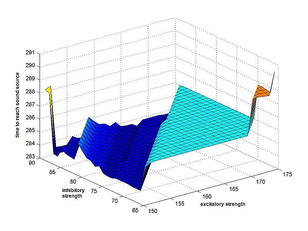
Important is that the valley floor of the time-results isn't as flat as it appears to be on the plot shown above (Fig.4b). This is clear when looking at Fig.5, which shows a close-up plot of the time-measure-surface.

Fig.5 Detail of the valley floor of Fig.4b, the time-measure-surface. This detail shows that the valley floor is less flat than it appears on the large plot. It shows that the surface is relatively uneven, and that there will not be one single minimum.

Fig.5 shows that there is more unevenness in the valley floor than is visible at first. It turns out that these differences are minimal, but noticeable in the cricket's motion: when running the program for different synaptic weights, one can see slight differences in the crickets movements, different, slightly longer turns seem to be taken. However, this difference is minimal, as can be seen in the movie-files downloadable below.

movie 1: Cricket motion for a cricket with excitatory strength = 16 and inhibitory strength = 7
movie 2: Cricket motion for a cricket with excitatory strength = 16.5 and inhibitory strength = 8.75

After these tests we decided to continue with the time as primary comparison criterion. We chose it because it is more intuitive than the angular delay, and the differences in the distance-measure aren't all equally important, as explained above.

Optimizing the parameter settings

Faze 1

To this point we had been able to note some of the possibilities of changing the synaptic weights, and we wanted to move to a higher dimensional parameter space. By testing some other pairs of parameters in 2D-space, we had discovered that probably all parameters are closely linked, and no small number of parameters determines the whole behavior of the cricket.

In the genetic algorithm described above, we had to make a few decisions on initializations.
We chose each cricket to have 5 variable parameters, to be optimized by the program: the 2 synaptic weights, tMemb (time constant of the membrane), tAdapt (time constant for the adaptation of the membrane) and Ginc (the amount of adaptation after a spike). These 3 last parameters were to be the same for all 4 neurons in the system.
As for the ranges of these parameters, we chose not to put any tight restrictions on any of them, although we had very strong suspicions that for example the synaptic weights would be between 15 and 30, etc. We preferred to let everything be discovered, be optimized by the algorithm itself. Thus, we chose the synaptic weights to have ranges from 0 to 45, tMemb from 0 to 10, tAdapt from 0 to 100, and Ginc from 0 to 0.06.
The mutation-probability was chosen in such a way that, on average, every two generations one of all parameters over the whole population would be mutated.
Finally, the last thing we had to choose, was the number of animals per generation, which we set at 12.

It turned out that every time the algorithm converged to one specific parameter setting. The amount of generations this took, however, was highly variable.

On every parameter setting that we got as result from the genetic algorithm, we ran extra tests: we tested them by running them on 50 random sound source positions. In general, the results were good, but none of the parameter settings resulted in the cricket reaching the sound source at every position tested. So probably the system is too much simplified to create a cricket that works well on all possible sound source positions. However, what these tests were really good for, was to get an idea of plausible parameter ranges for all parameters, instead of the very general ranges we started with in our optimization algorithm tests.
We ran all of the crickets, generated by the genetic algorithm, against the same large set of random angles, to compare them. We calculated what percentage of the tests were successful (in what percentage of the tests the cricket actually reached the sound source), by using the time-measure. We also used the distance-measure, calculating the average minimal distance over all successful tests, and the average minimal distance over all unsuccessful tests, for all crickets. From the data collected from these tests, we decided which cricket gave best results overall, and designated that cricket as "species A". All the tests done so far, were done with input sounds consisting of bursts, interleaved with intervals of length 40 ms. (see Table 1)

Then we did the same optimization procedure again from the start, with inter-burst-intervals 50 and 80. This way, we wanted to check the possibility of creating new "species" of crickets, using the same system, and only changing the 5 parameters we had varied so far. We wanted to know to what extent the behavior would change, and how different the parameters would be.

The procedure was exactly the same, and thus we ended up with 3 optimal crickets, 3 different species: a 40-cricket, a 50-cricket and a 80-cricket. To compare them, we ran each of these crickets on a wide range of random angles (again), for various inter-burst-intervals.
This was done to test 2 basic properties:
- whether each cricket would effectively be the best of the 3 on its own "trained" inter-burst-interval
- whether each cricket would better on its "trained" interval than on all other intervals.
The results are shown in Table 2.

So now the question was whether this obvious lack of combining power for selectiveness and good performance was inherent in the system, or whether it could be solved my making the system slightly more complicated, without changing anything to the initial construction.
So we changed the number of parameters per animal from 5 to 8, by making tMemb, tAdapt and Ginc different for AN1 and MN neurons. So both AN1 neurons would still have the same values for these parameters, but these could be different from the values for the MN neurons. We ran the whole optimization scheme again for the worst species so far: the one with inter-burst-interval 80; the results for the cricket are listed in Table 3. Now the overall performance is better, but the interval of length 80 is not the optimal interval anymore. So we gained on one property, but lost the other.

Faze 2

Initially, we wanted to try to get a good working system with as few changes as possible.

First we took the parameter setting from the optimal cricket we had gotten so far for an inter-burst-interval of 40 ms (see Table 2). We gave the ON1 neurons the same parameter values as the other types of neurons, and they were all fixed. Then we searched in 3-parameterspace by making the synaptic strengths of the connections the only variables: the excitatory AN1-MN weight, the inhibitory ON1-ON1 weight and the inhibitory ON1-AN1 weight. But no good results came of it.

The following is meant by "no good results":
We let the genetic algorithm run, and let it print out it's results after each generation. In each generation all crickets were tested against 5 different sound source angles.
Most times, we got just all values 600 for all crickets (= the crickets never reaches the sound source). Sometimes, we got something around 570 or so for all crickets: this means that 1 of the 5 angles tested at that generation was so small, that all crickets, although only moving straight or turning very slightly, still would reach it fast. Averaging one fast time with 4 600-times would give a value between 500 and 600.
If after 3 generations, there was no distinction between the different crickets, and all values were bad in all 3 generations, we interrupted the run, and restarted with a new one. This would result in better chances of getting a good-performing cricket.

Secondly, we moved to a 6-parameter space, by making tMemb, tAdapt and Ginc variable too. we used the same values of these parameters for all 3 kinds of neurons.
Again, no good results came out of the genetic algorithm.

As a third test, we moved to a 9-parameter search, by splitting tMemb, tAdapt and Ginc up: AN1 and ON1 still got the same values (since that idea is supported by data from [7]), but MN's values could be different.
Again, no good results.

For each space (3, 6 and 9) we did about 5 to 10 of these tests, none of them were any good.
Once in 9-parameter space, it seemed to work better, so we let it run to 8 generations. After that, there were 2 crickets left, that seemed equally good.
But when we let them both run against 50 different angles, it turned out they both only reached the source in about 8% of the cases. So it wasn't any good after all, especially when comparing this result to the results we got in the more simplified system.

We figured that something else must be changed to get the algorithm to converge to a decent-working parameter setting.
One thing that seemed logical was to use delays: up until now, the excitatory input from the ears to the AN1 and ON1 arrived at the same time. But this also means that the inhibitory effect of the sound to AN1 is delayed (because it has to be processed first by ON1.
So what we tried is to delay the excitatory input from the ears to the AN1 by a certain number of time steps. That way, inhibitory and excitatory inputs would arrive at AN1 in a variety of time-differences. We tried delays of 1,2,3 and 5 time steps.
None of these modifications improved the results we got in a considerable amount. There was one parameter setting, at a delay of 2 time steps, that seemed to work better than previous tests. But after running that setting against 50 different angles, it still only got to about 16% of the sound sources, which is still a poor result, when compared to the percentages we got in our more simplified system.

• eicricket.m: Example cricket where the numerical integration was implemented using Euler's method with linear interpolation; it returns the minimal distance as result.
• anglecricket.m: Analogous cricket as 'eicricket.m', but returning the angular delay as result, instead of the minimal distance.
• movingcricket.m: Analogous cricket, generating more output: it shows the movement of the cricket throughout the computations, and shows output for the 4 different neurons in the system (potential, adaptation, spike train).
• mostparams.m: Most detailed cricket we optimized with the limited system, using the genetic algorithm.
• genetic.m: Genetic algorithm to optimize the parameters of a cricket (in this file: mostparams.m).
• testbursts.m: Example program to test a certain cricket against a large number of sound source positions over a wide range of inter-burst-intervals.
• newcricket9.m: Most detailed, biologically more correct, cricket from faze 2, with 9 parameters.