Damian Elias and Bruce Land.
Introduction
Neurobiologists and people studying animal behavior often want to measure and classify visual stimuli (1). Characterizing the motion of a stimulus for comparision with other stimuli is not well defined at present. We are attempting to figure out a scheme for measuring the motion properties of a motion sequence. The goal is to summaried the motion in a way with conveys the essential aspects of the motion, without overwhelming the investigator with detail. The first application is in spider visual courting displays.
Methods
There are several ways of estimating motion. The two basic approaches are object based (e.g. 2) and image based methods. Object based methods use information about the 3D geometry of the structure generating the motion to estimate parameters such as joint rotation or limb velocity. Image based methods use only the information that might be available from a single video tape, or that might be observed by an animal under test. We chose to concentrate on image based methods because we need to compare video sequences of spider behavior.
The image based scheme we used had several processing steps
I is the array of intensities
at every point in a frame, and v is the vector velocity of the
object seen by the pixel, thendI/dt = -∇I dot vvg = -(dI/dt)∇I /mag(∇I)2
For each frame, the total pixel motion was estimated by averaging
the speeds of all pixels. The "average speed" of a frame was a simple
average of the magnitude of v of all the pixels in the frame, as used by Peters,
et al on motion studies of the Jacky Dragon. We also defined a "speed
surface" (consciously trying to mimic the usefulness of a spectrogram).
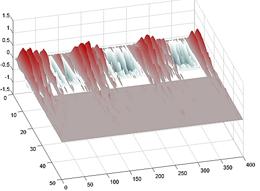
The speed surface is a 2D plot with the x-axis being frame number, y-axis
being pixel speed, and the color proportional to the log of the number of
pixels moving at a given speed. In other words, at each frame time we plotted
a histogram of pixel speeds.
The programs
The following matlab programs implemented the various features noted above.
Step 1 above was carried out by a short program that reads an AVI file, selects a frame range, and writes a MAT file containing a Matlab movie.
Step 2 and 3 are carried out by a program which takes as input the MAT file containing a movie, decimates the resolution, builds a 3D array (x,y,t) of images, normalizes the intensites, computes the motion and outputs two files, containing respectively arrays of speed and speed histogram (speed surface). Each individual analysis to 2 to 15 munutes on a 2.6 GHz Pentium with 1Gbyte of memory.
Step 4 and 5 is carried out by a program which takes as input the arrays from step 3, pads the sequences to the same length, computes the circular cross-correlation for each pair of signals and forms a distance matrix repesented the dis-similarity of all possible signal combinations. The entropy is then computed as in Victor and Purpura (4). There were actually two versions of this program, one for the Hpug data and one for the Hdos data. The only differences were the hard-coded file names and group indices.
Step 6 is carried out by a program modified from reference (5). The MDS is computed, then a-priori groups are marked with different colors. In addition, this program carried out an ANOVA along a selected axis of the MDS analysis. There were actually two versions of this program, one for the Hpug data and one for the Hdos data. For both data sets, a 3D fit was used. With ANOVA performed along axis 1, and for Hpug data along axis 3.
Examples of Analysis results
All of the files resulting from step 3 are available. The zipped version is here. The
files with names starting with Fake represent calibration files
not actually used in the final analysis. The file names which include gram
are 2D histograms. The dimensions are time and speed bin, and the values are
number of pixels in the speed bin. The file names whih include wave
are 1D average speeds, with the dimenson being time.
Habronattus pugillis (Galiuros)
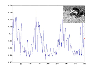
The following image is a link to a matlab movie with animated speed trace. In the movie, you can see the correlation between average pixel speed (blue line) and leg motion (inset). Frame number is on the horizontal axis, average speed on the vertical axis. Movie size is 2.5 MByte. The spider is Habronattus pugillis (Galiuros).
The following images are the 2D speed surfaces for Habronattus pugillis (Galiuros) There are two versions shown. The first is a 2D histogram with red indicating a large number of pixels at the given speed and black indicating a low number of pixels. The second projects the histogram into a 3D surface.

Habronattus pugillis (Santa Catalinas)
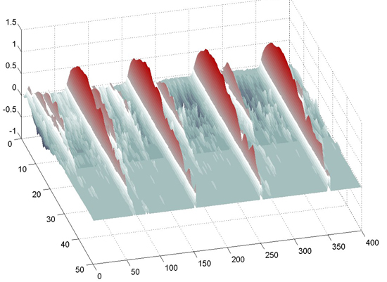
The following three images (first is a link to an animation) show data from another species whcih has a dramatic leg-flick.

MultiDimensional Scaling
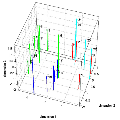
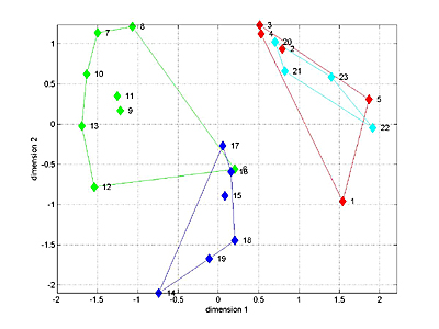
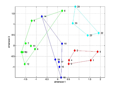
The 1D speed traces and 2D speed surfaces were analyzed by computing the maximum cross-correlation between each pair of signals, for a total of 23 signals. This resulted in a 23x23 matrix of "similarities" bewteen signals. MDS attempts to find a low-dimensional space which adequately captures the (potentially) high-dimensional nature of distances between signals. For distance we used (1-similarity) of the 1D speed traces. A 3D fit seemed to capture most of the variation between signals for the four Habronattus pugillis variants we tested. A 3D plot is shown below with the four variants in different colors. The next two images show two projections of the 3D data. It is clear the the 4 groups can be separated in 3D. Analysis of variance along the relevant axes confirm the significant separation.
Links to manuscript and figures submitted in Sept 2005.
References