Introduction
This project implements a real-time scrolling spectrogram-style visualization of an audio signal. We successfully displayed the frequency spectrum content in real time using a 4-bit grayscale scrolling display on any NTSC television. The frequency spectrum of an audio line-in input or mic input is calculated and displayed in real time using two ATmega1284 microcontrollers units (MCUs). Features include play/pause functionality, slowing down scrolling speed by factor of 2,3 and 4, as well as displaying in linear or log scale. Each MCU handles separate tasks:
- The Audio MCU performs data acquisition and performs audio processing.
- The Video MCU performs the visualization processing and video output to NTSC standards.
A male-to-male 3.5mm audio cable, the user can connect any audio producing device such as a computer or MP3 player to the device’s 3.5mm audio jack and input an audio signal. Using a male-to-male 0.5mm video cable, the user can connect any standard NTSC television supporting resolutions of at least 160x200 to the device’s 0.5mm video jack and see the frequency spectrum of the input audio signal on the TV.
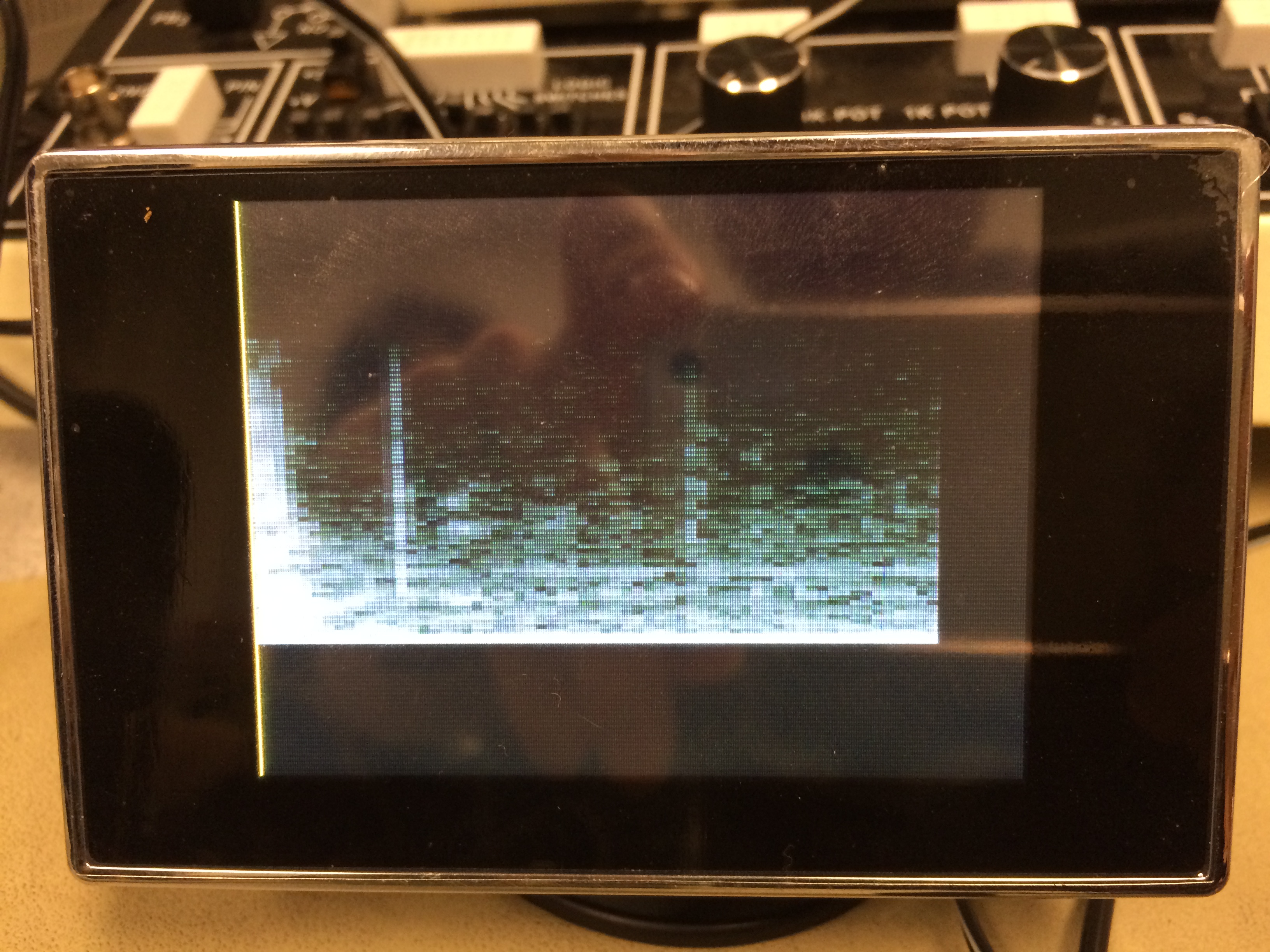
The device can display audio frequencies up to 4 kHz. This range covers the majority of the frequency range of typical music. An example spectrogram output is shown below.
High Level Design
Rationale and Source of Idea for Project
Early in the semester, we thought about building a real-time speech recognizer which takes the input from a microphone, analyzes it through FFT conversion, and displays how close two different audio inputs are to one another. We quickly determined that this was a very hard problem to solve within a 5-week period. However, we then determined that we may be able to display audio as a real-time spectrogram, and determine the "similarity" of two audio inputs by analyzing the spectrograms by ourselves. We also noticed that a similar project was carried out under the name "Audio Spectrum Analyzer" by Alexander Wang and Bill Jo, which we referenced quite often throughout the project.
Logical Structure
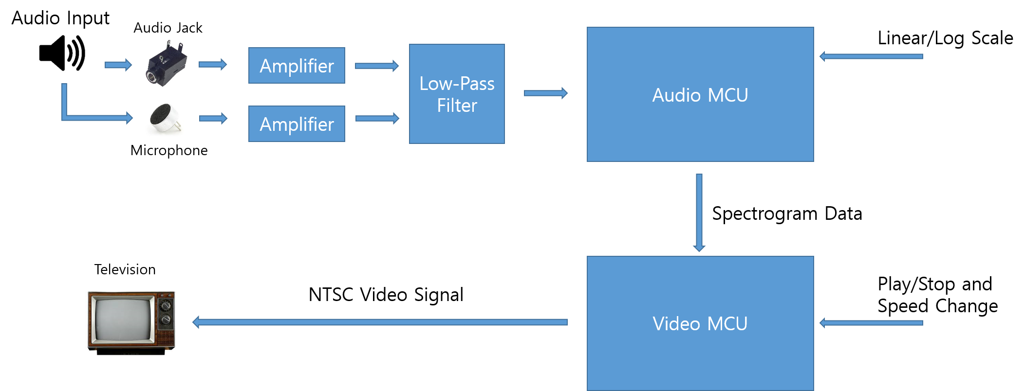
The data flow of the project is linear. First, the audio signal is received from either of the sources; audio jack or a microphone. Then the received signal is level shifted to add a DC bias voltage and then amplified. The amplified signal is sent through a low pass filter with a cut-off frequency at 3KHz. The signal is then fed to the ADC (Analog to Digital Converter) in the Audio MCU which samples the signal at 8KHz and converts it into a digital signal. A Hanning window is applied on the output signal of ADC. Then, the signal which is now a discrete set of 128 points is converted to a frequency domain using a 128 point FFT (Fast Fourier Transform). This frequency domain data is transmitted to the Video MCU through USART. The Video MCU processes the received data into a scrolling 4-bit grayscale histogram visualization in real-time. Finally, the Video MCU transmits the video signal to the TV. The user controls push buttons to play/stop, change speed of scrolling, or change the frequency magnitude scaling.
Tradeoffs between Hardware & Software
The main hardware and software tradeoff was in deciding whether to use a single MCU and complicate the software or to use two MCUs and add a little extra hardware that distributes software complexity between the two MCUs. Since the calculation of the frequency spectrum and the NTSC signal generation each take up a significant portion of the CPU power, we decided to use two ATMega1284p CPUs, each dedicated towards frequency analysis and video generation. The tasks of acquiring data and processing it will be handled by one microcontroller, while the other will perform the tasks required to display the actual visualization. This decision is also made by taking into consideration that all the operations need to be done in real time which require precise timing i.e., the audio sampling of the input audio signal need to be done at precise intervals, and also the data transfer and processing in the video MCU should be done during the “blank lines” of the TV. So, we decided to use two MCUs.
Components & Standards Compliance
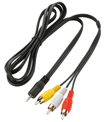
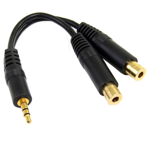 Several hardware and communication standards are used in the project. Regarding hardware standards, a standard 3.5mm stereo audio jack socket and a microphone to take in analog audio signal are used. The audio jack is intended to connect to a TRS (Tip, Ring, Sleeve) type male audio connector. The same connector is used to output video signal to the NTSC Television. Since most televisions use the RCA headers, we use a 3.5mm-audio-to-RCA cable shown below. We also used a splitter (left) to connect the input signal from the audio jack to the device as well as to the speakers.
Regarding communication standards, we used the NTSC analog television standard to output 4-bit grayscale video to a NTSC compatible television. NTSC (National Television System Committee) is the analog video standard used in most of North America. This standard defines the number of scan lines to be 525, two interlaced fields of 262.5 lines, and a scan line time of 63.55uS. The standards set by NTSC are closely considered in our project when creating the video signal to output to our TV.
While not technically a standard, we also used USART to serially transmit data between the two MCUs. The Atmel Mega1284 MCU has various frame formats that must be followed in both the transmit and receive MCUs including synchronous mode which we used.
Mathematical Background
Determining the Sampling Frequency
The sampling rate or sampling frequency defines the number of samples per second (or per other unit) taken from a continuous signal to make a discrete signal. The Nyquist–Shannon sampling theorem states that perfect reconstruction of a signal is possible when the sampling frequency is greater than twice the maximum frequency of the signal being sampled. If lower sampling rates are used, the original signal's information may not be completely recoverable from the sampled signal. The highest frequency component in the audio input signal is around 4kHz when we consider a 3kHz cutoff frequency with an 8-th order low-pass filter. So, according to Nyquist–Shannon sampling theorem the sampling frequency should be greater than 8KHz. We considered 8KHz as the sampling frequency which triggered an ADC conversion once in every 2000 cycles (Frequency of CPU is 16MHz).
The Fourier Transform
The Fourier transform is a mathematical algorithm that converts a time domain signal into its frequency representation. Based on whether a signal is continuous or discrete and periodic or aperiodic, there are four types of Fourier transform. Fourier Transform (Aperiodic-Continuous signal), Fourier Series (Periodic-Continuous signal), Discrete Time Fourier Transform (Aperiodic Discrete signal) and Discrete Fourier Transform (Periodic-Discrete). As the project deals with finite digital systems, we used the Discrete Fourier Transform (DFT) which converts a discrete time audio signal of a finite number of points N into a discrete frequency signal of N points,. With a purely real-valued signal such as the input audio signal, the frequency representation of the signal is mirrored perfectly across the (N/2)th point in the DFT.There are multiple algorithms that calculate the result of the DFT quicker than calculating the DFT directly using its defined equation (while maintaining the same exact result), called the Fast Fourier Transform or FFT. Many FFT algorithms exist, but the majority of them use recursive divide-and-conquer techniques that reduce the O(N2) computation time of the DFT to O(Nlog2(N)). With a large N, this increase in speed is very significant in reducing computation time especially in software applications. Because of its recursive nature, it is usually necessary for N to be a power of 2. We use a fixed-point number based decimation-in-time FFT algorithm adapted from Bruce Land in our software to convert the discrete digital audio signal into discrete frequency domain.
Hardware
Audio Amplifier and Filter Circuitry
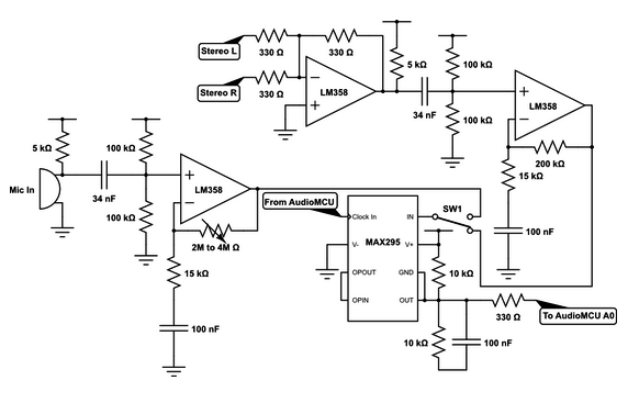
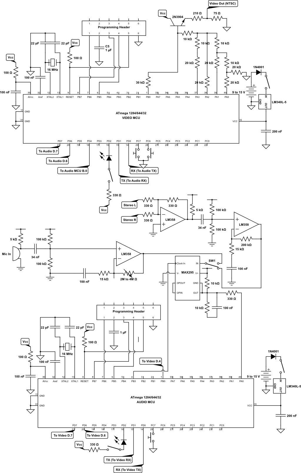
The audio amplifier circuit simply accepts a stereo line-in signal, a microphone audio input signal, and a 150 kHz input clock signal. The line-in and microphone inputs have separate gain stages using Texas Instruments LM358 op-amps, and a mechanical switch selects one of the two signals to feed to the 8-th order low-pass filter. The low-passed signal is then fed to the ADC through a 330Ω resistor.Since the ADC cannot read negative voltages, we had to decide a bias voltage for our audio input. We chose this bias to be 2.5V so that it sits between 0V and Vcc, due to simplicity of design - it was very easy to set the Analog reference voltage of the ADC to Vcc, and the 2.5V bias voltage was also a convenient value for our low-pass filter. To achieve this bias, the inputs from the microphone and stereo line-in are DC-biased to 2.5V with two 100kΩ resistors and two 17nF capacitors in series. the resulting biased signal is then amplified through a non-inverting amplifier circuit with high-pass cutoff frequency at 100Hz. The high-pass cutoff frequency was chosen such that the DC bias voltage would not be amplified by the non-inverting amplifier. This is also the reason for choosing the specific value for the capacitors at the biasing stage, since the high-pass cutoff frequency of the level-shifter should match with that of the amplifier circuit.
On the line-in amplifier specifically, the stereo line-in’s left and right channels are fed through a summing unity-gain inverting amplifier, which is then fed through the biasing circuit described above. The biased output is then fed through an AC-coupled non-inverting amplifier. To determine the gain of the amplifier, we experimented with the line-in output and observed that the maximum voltage swinge was 2V peak-to-peak. Thus, we determined that a gain of ~6V/V was adequate so that the user could output audio on a reasonable volume level and still have significant signal strength going to the ADC. Our final gain based on our components was 6.67V/V, or +16.48 dB.
Similar to the line-in circuit, the mic-in circuit runs the input from the microphone through the biasing circuit. This signal is then passed through a non-inverting amplifier with a 4MΩ resistor on the negative feedback loop. As with the line-in circuit, this value was chosen after experimentally determining the maximum voltage swing of the mic-in audio to be around 20mV peak-to-peak. Thus, to be able to detect voices of reasonable strength and distance away from the microphone, we chose the above resistor value to obtain a gain of 266.67V/V, or +48.5 dB. This ensures that the maximum output of the microphone results in a full voltage swing across the ADC range.
Since we sample the audio signal with the ADC at 8kHz sampling rate, we must low-pass filter the audio signal before the ADC conversion to remove aliasing. To preserve as much of the signal below 4kHz as possible, we must have a low-pass filter with high rolloff so that we can put our cutoff frequency as close to 4kHz as possible. We could have easily designed a 2nd-order low-pass filter - such as a Sallen-Key Filter - but it would not be enough since a 2nd-order filter has a rolloff of -20dB/decade, so for 90% attenuation we need to have cutoff frequency at 800Hz, which is too low for us. Thus, we decided to use the MAX295 8th-order low-pass Butterworth filter which has a moderately steep slope (among other various 8th-order filters), has flat pass and stop-bands, and has relatively linear phase shift so distortion is minimized.
As shown in the schematic below, a clock signal generated by the Audio MCU determines the cut-off frequency of the low-pass filter, which is set at 3kHz. Clock to corner frequency ratio is 50:1, so the microcontroller feeds a 150kHz clock signal with Timer 0 to achieve 3kHz cutoff. Note that 3kHz was chosen as the cutoff frequency since we wanted to preserve more of the higher frequencies even if it meant having a little bit of aliasing in our audio signal.
Shown below are the resulting amplification of the actual circuit. Note that Line-in amplifier has gain of ~6V/V and the microphone amplifier has gain much higher gain, but is unmeasurable due to high-frequency noise content in the original signal.
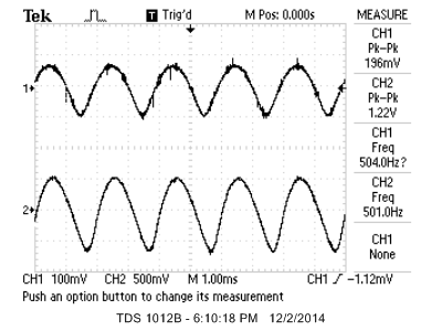
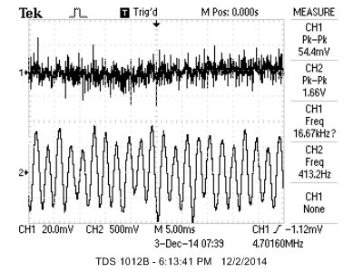
We also measured the behaviour of the low-pass filter. At 2kHz signal was attenuated, at 3kHz signal was attenuated to half amplitude, and at 4kHz signal was attenuated to ~1/8 the original amplitude, which matches with our design of 3kHz cutoff frequency.
Push Button Circuitry
The push button circuits are simple debounced push buttons that toggle the play/pause, speed control, and log/linear conversion functionalities for the audio and video microcontroller units. The basic button input circuit is shown below. The 330Ω resistor is designed to protect the input pin of the microcontroller.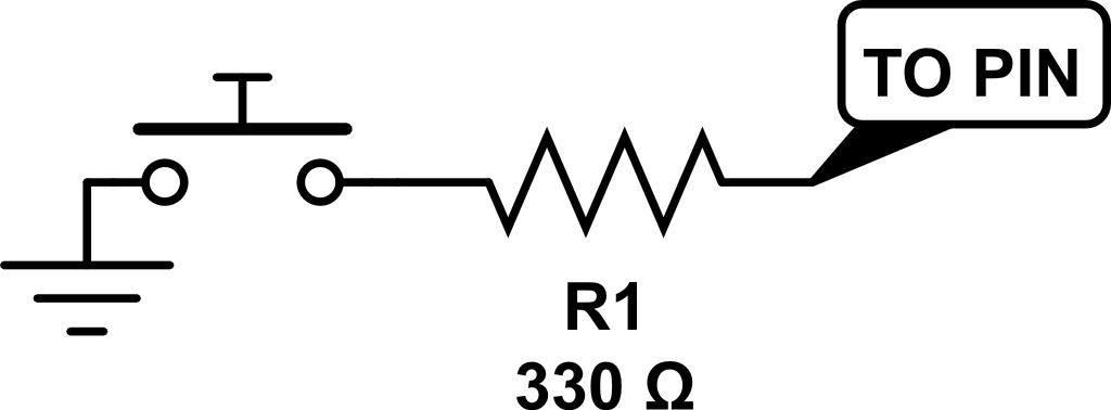
Audio & Video MCU Connections
The Audio and Video MCUs communicate via USART in synchronous mode. The Audio MCU uses USART0, and the Video MCU uses USART1. Thus, we connect Pin B.0 of Audio MCU to Pin D.4 of Video MCU for the clock signal, and the Tx pin (Pin D.1) of Audio MCU to the Rx pin (Pin D.2) of Video MCU for actual data transmission. For flow-control of data, we connect pin D.6 and D.7 of each MCU to each other to carry receive/transmit carry signals. The details of how they are actually used is discussed in the Software section. Please refer to the hardware schematic in the Appendix for the exact wiring between the two MCUs.
16-bit Gray-scale Video Generator
For 16-bit grayscale generation we borrow the circuit built by Francisco Woodland and Jeff Yuen in their Gray-Scale Graphics: Dueling Ships final project. As can be seen in the schematic below, we use a R-2R resistor ladder network to add the 4-bits representing grayscale intensity and the sync signal. The added voltage is passed through a common collector circuit that serves as a voltage buffer, and the resulting voltage is shifted to 0V ~ 1V range by a 210Ω/75Ω voltage divider. Pins A.0 to A.3 are connected to bits 0-3 of the resistor ladder, and pin B.0 is used to drive the sync signal.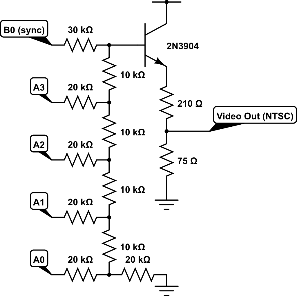
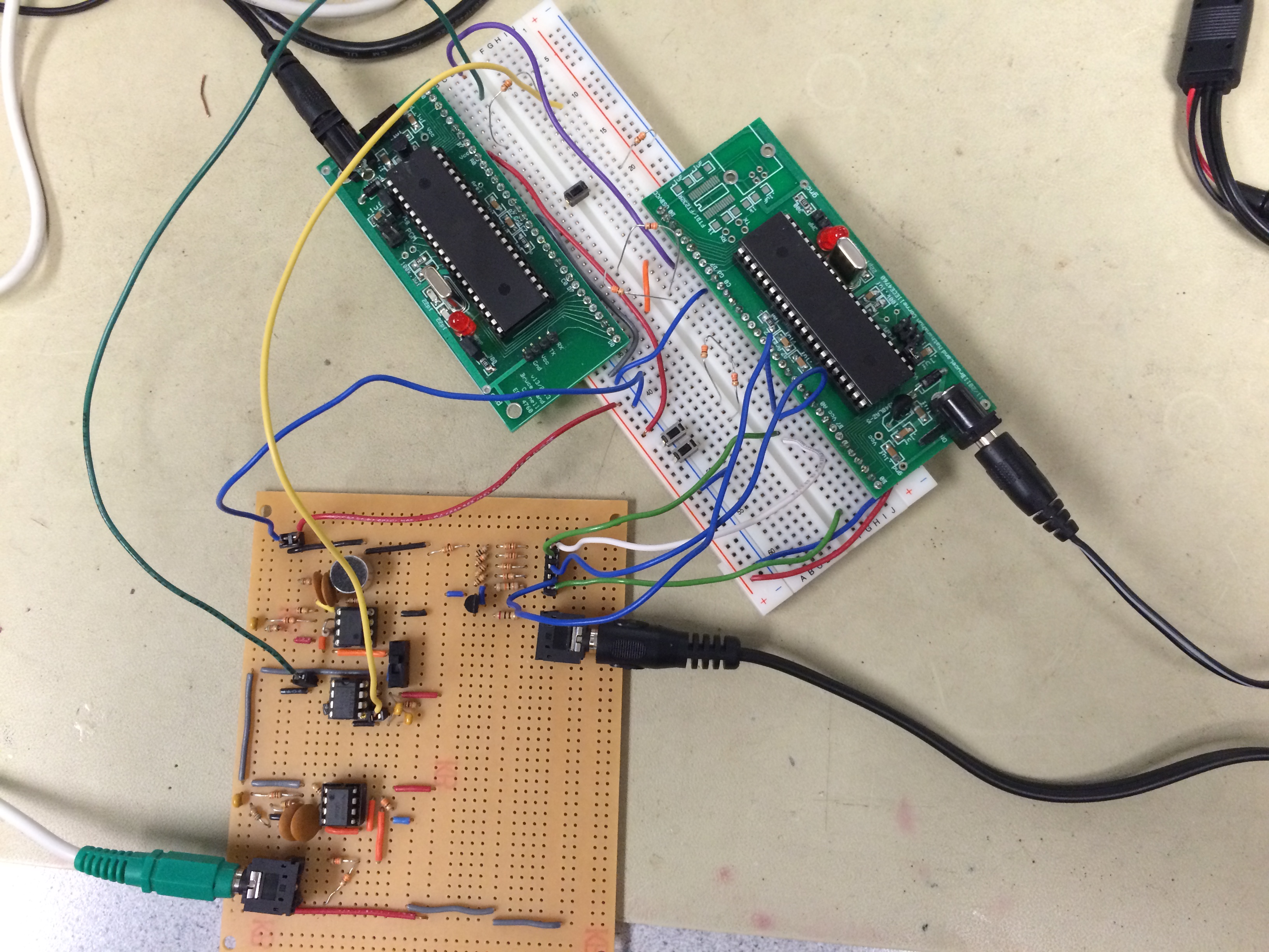
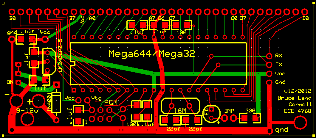
Hardware Implementation and Integration
Since we use two MCUs, we have both MCUs on their own target boards. Since we salvaged the Video MCU and its target board from the lab, its target board schematic is a bit different from the target board of the Audio MCU, but the difference is ultimately irrelevant in the operation of our spectrogram. The target boards and push buttons are mounted on a single breadboard to allow easy connection between the two MCUs. The MCUs also share a common ground, but use separate 9 or 12V power supplies. The audio amplification and filtering circuit is soldered on a separate solder board since it has many more components, with pin sockets soldered for easy wiring between the MCUs and the circuit input/outputs. There are also two 3.5mm line-in jacks soldered for inputting audio and outputting video to the television. The final hardware wiring is shown below.
Software
The software portion of the project was split in two between the code for the Audio MCU and the Video MCU. The audio MCU is responsible for the audio data acquisition, converting the analog audio signal into digital signal by ADC sampling, converting the digital time domain signal into frequency domain using FFT and transmitting the processed data to Video MCU through USART. The Video MCU is responsible for receiving the data from the Audio MCU through USART, performing the visualization processing by using 4-bit grayscale, implementing a circular buffer to get a scrolling display and transferring the data to the NTSC television. The FFT part in audio MCU and the video display part in the Video MCU were based off of the example code shared by Bruce in the public course website. Regarding the software setup, AVR Studio 4 version 4.15 with the WinAVR GCC Compiler version 20080610 was used to build and write the code, and to program the microcontroller. The crystal frequency is set to 16 MHz and compiler optimization was set to -Os to optimize the speed.
Audio MCU
ADC Sampling of Audio Signal
The modified audio signal from the audio analog circuit was fed into the ADC port A.0. The ADC voltage reference was set to AVCC. By default, the successive approximation circuitry requires an input clock frequency between 50kHz and 200kHz to get maximum resolution (according to the Atmel Mega1284 specifications). So, the ADC was set to execute at 125 kHz to allow 8 bits of precision in the ADC resulting value, which we deemed sufficient for the project. In order to get accurate results, we must make sure to sample the ADC port at precisely spaced intervals. Since the ADC is running at 125kHz and it takes 13 ADC cycles to produce a new 8-bit ADC value (ranging from 0-255), or about 104us. The ADC was set to “left adjust result”, so all 8 bits of the ADC result were stored in the ADCH register. At a sample rate of 8kHz, an ADC value will be requested every 125uS, which means there should be sufficient time for a new ADC value to be ready each time it is requested. The sample rate was set to be cycle accurate at 8 kHz by setting the 16 MHz Timer 1 counter to interrupt at 2000 cycles (16000000/8000=2000), and having the MCU interrupt to sleep at 1975 cycles (slightly before the main interrupt) to ensure that no other processes would be interfering with the precise execution of the Timer 1 ISR where the ADC is sampled. The output from the ADC was stored in bits 2 to 9 of a 16-bit fixed-point integer buffer on which hanning window was applied. Then it is used as input for the FFT.
Fast Fourier Transform
After waiting for 128 samples of the audio signal, FFT conversion begins in the main loop of the program. We use the FFT conversion method provided for us by Professor Bruce Land, which takes real and imaginary input arrays of size N (where N is a power of 2) and calculates the resulting real and imaginary frequency vectors in-place. Since the resulting array contains both positive and negative frequencies symmetrically, we use only the first 64 entries of the array.Following the conversion, we calculate only the magnitude of the frequency, since phase is not used. Since taking a square root of the sum of the squares is too costly, we use the following approximation to calculate the magnitude:
Magnitude of k-th element = Max(frk , fik) + 0.4*Min(frk , fik)
Where frk represents the k-th element of the real vector and fik represents the k-th element of the imaginary vector. As shown in the “Function Approximation Tricks” page, the above approximation has an average error of 4.95%. This is acceptable since our frequency magnitude resolution is already so low (only 16 discrete values), so the magnitude calculation error is insignificant compared to the quantization error.
The calculated magnitude is then divided into 16 discrete levels by linear or base-2 logarithmic scaling, according to the user’s choice. With linear scaling we take the middle 8 bits of the 16-bit fixed-point value (bits from 4 to 11) and then assign a value to a new char array that contains the scaled values. With base-2 logarithmic scaling, we use the position of the most significant bit of the magnitude as the logarithmic value to store in the char array. For example, a magnitude value with the most significant bit at position 5 would be approximated as log(magnitude) = 5+1 = 6. After discretization is done, the 64 bytes of frequency values are transmitted to the video MCU via the USART data transmission protocol. This is discussed in detail in the following section.
USART Data Transmission & Reception
For transmitting data from the audio MCU to the video MCU, we use the USART data transmission and reception protocol. The USART protocol uses two wires for transmit and receive, and an additional wire when using synchronous mode. We opted to use USART in synchronous mode since synchronous mode provides the fastest data transfer rate, since the additional clock is used to check the integrity of the communication whereas the asynchronous mode requires additional overhead in checking data integrity. We use USART channel 0 on the audio MCU to transmit the frequency magnitude data to the video MCU, and USART channel 1 on the video MCU to receive the transmitted data. We chose USART channel 1 instead of 0 on the video MCU since we originally used channel 0 to output black-and-white NTSC signal to the television.Both USART are set up to transmit 8-bit size characters, with a start bit and a stop bit to signal the start and end of a character. Thus, a frame consists of a total of 10 bits. Since both USART are operating in synchronous mode, we set the Baud rate of the transmission by the following equation:
Where fosc is the CPU clock frequency. Since the external clock frequency has to be less than a quarter of the CPU frequency - which is at 16MHz - the maximum BAUD rate we can achieve from the above equation is 2MHz, which we achieved by setting the register UBRR0 = 3. Since we can keep sending data at every clock edge as long as we keep the USART Transmit Data Buffer register full at all times, we thus calculate the maximum data transfer rate as:
![]()
A major hurdle in USART communication was flow control - namely, when to start/stop sending data to the video MCU. Notice that when the video MCU is busy drawing the visible lines on the television, it does not have time to accept data from the audio MCU. Thus, we must ensure a correct flow control scheme where we only send data when the audio MCU is ready to transmit (i.e. has all the frequency magnitudes calculated) and the video MCU is ready to receive (i.e. drawing blank lines on screen).
To achieve this, we adapt the flow control scheme used by “Audio Spectrum Analyzer” final project of Alexander Wang and Bill Jo (Fall 2012). We use Pin D.6 as the “transmit ready” pin that the audio MCU controls, and Pin D.7 as the “receive ready” pin that the video MCU controls. When the audio MCU is ready to transmit, it sets the transmit ready pin HIGH and waits for the receive ready pin to go HIGH. When the video MCU is in turn ready to receive, it will set its receive ready pin HIGH, and the audio MCU starts transmitting data. Note that the audio MCU cannot send data indefinitely since the video MCU has to put out a sync pulse every 63.625 us. Thus, we designed the audio MCU to send 4 bytes of data per video line timing, which requires a total of approximately 20 us considering the stop/start bits. When the video MCU starts receiving the data per line it immediately lowers the receive ready pin so that the next 4 bytes are not sent until the next line. After all 64 bytes of data have been transmitted, the audio MCU sets the transmit ready pin LOW and waits for the new sample data.
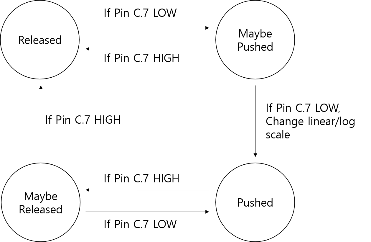
Linear/Log Scale Button
We wanted the user to be able to choose whether he/she wanted to view the spectrogram in a linear or log scale. Thus, we created a simple de-bouncing state-machine which changes its state given a push button input. The push button connected to pin P.7 is active low, with an internal pull-up resistor turned on at the pin. Every time an FFT conversion is needed, the system polls the input at the pin and de-bounces the input by going through a "de-bouncing" state. If the input is considered valid after de-bouncing, the display state is changed between linear and log scale. A diagram of the state machine is shown below.
Video MCU
NTSC Video Generation
The video MCU is responsible for taking the received frequency values and displaying them in a gray-scale scrolling spectrogram on a NTSC television. Since the NTSC protocol has been discussed in extensive detail in Lab 3, we will only discuss the fundamentals needed to understand our project.A television operating on the NTSC standard is controlled by periodic 0-0.3V sync pulses which determine the start of video lines and frames being displayed. One can imagine a single trace moving across the monitor in a "Z-pattern" along each line. Although the standard dictates drawing 525 lines in 30 frames per second, one can choose to display only half of the lines (262) at 60 frames per second. This results in a 63.5μs video line timing. Although the exact timing may vary by about 5%, it is crucial to have the timing be consistent. After a sync pulse, a voltage level ranging from 0.3V to 1V determines the black/white level of the display, where higher voltage results in a whiter image.
For accurate sync generation, we use the coded provided for us in Lab 3 by Professor Bruce Land. We use Timer 1 to generate the sync signal by entering the COMPA interrupt service routine every 63.625μs. Since one can only enter the interrupt after finishing the execution of the current instruction, this results in a 1~2cycle inconsistency in our video line timing. To prevent this, we set OCR0B such that we enter the COMPB ISR just before the video line timing to put the CPU to sleep. Since it alwasy takes the same amount of cycles to wake up from sleep mode, this ensures consistent video line timing.
Receive Buffer
When receiving the 64 frequency magnitudes from the audio MCU, the video MCU stores these values in a temporary receive buffer. The receive buffer (named receiveBuffer in code) is a 64-byte size char array, with each element storing the magnitude of each frequency bin. After the receive buffer is filled, the content of the buffer is copied to the Circular Screen Buffer for displaying to the television screen.
Circular Line Buffer
To have a scrolling spectrogram, one must display the contents of the Receive Buffer as a column of grey-scale “intensities” on the rightmost side side of the television screen, while shifting the older data left by one. In the television display code we were originally provided for Lab 3, we have a single screen array of size bytes_per_line*screen_height. Thus, the single screen array acts as a combination of multiple screen line buffers, where each line buffer immediately follows the previous line buffer. We originally considered copying the elements of each line buffer left by one, and then saving the frequency intensity at the rightmost element of each line buffer. However, we determined this to be too costly, since we only have a very limited time until we have to display the next frame.To solve the scrolling problem efficiently, we use circular line buffers. For each line buffer in the screen array, we keep track of a “start” pointer of the buffer. When a new frequency magnitude value is to be added, we add it at the position the pointer is indicating, and then move the pointer right by one. When we need to actually display the content of the buffer, we start displaying from the element the pointer is pointing at, and end at the element left of the pointer. Thus, as shown in the diagram below, we can efficiently shift the position of each data relative to the buffer’s starting position without doing any actual data shifting.
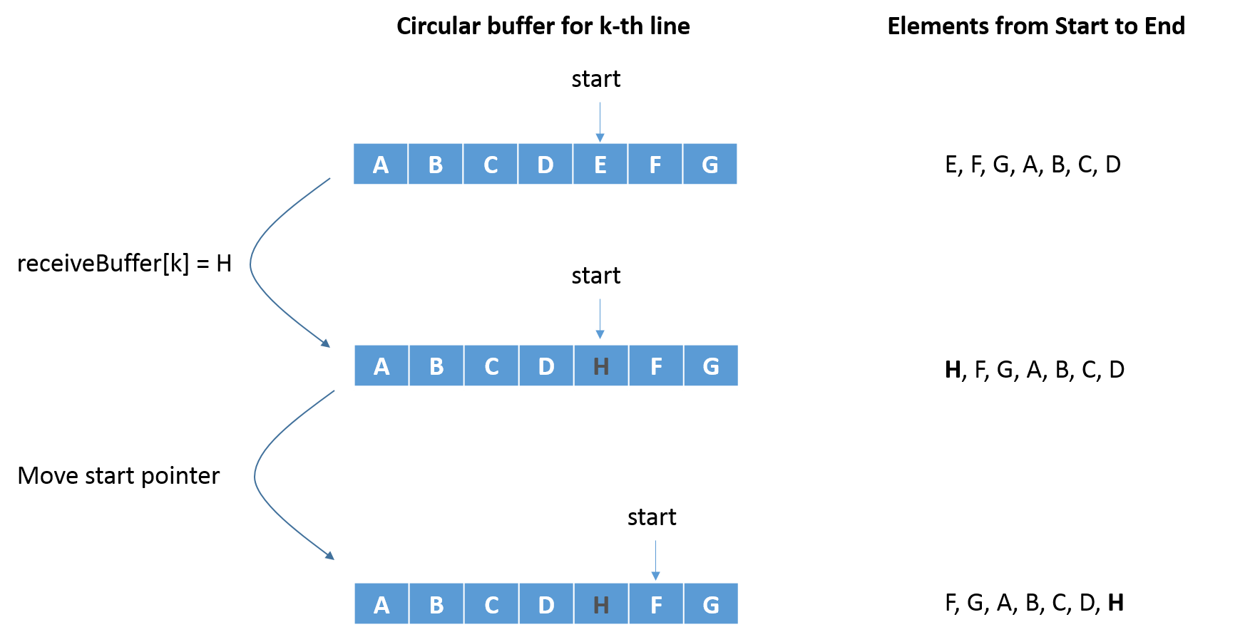
Traditionally, spectrograms display higher frequencies on higher horizontal positions. Our implementation of displaying on the NTSC television numbers lines from top to bottom - i.e. lines on higher horizontal positions are lower in number. Thus, we save the k-th element of receiveBuffer on lines 156 - 2*k and 157 - 2*k. These values are obtained by calculating (bufferSize - k - 1)*2 + 30, which maps the lower frequency values (lower k) to lines of higher value (lower in horizontal position). Note that we save a frequency magnitude in two adjacent lines, so that the user can distinguish different frequencies more easily.
Note that since all line buffers are of the same size, and they contiguously compose the screen array, we only need keep track of one starting pointer - in our implementation the starting pointer of the first buffer called screenArrayPointer - and calculate the rest using the relative positions of the circular buffers within the screen array.
Grayscale Display to Television
As explained in the Hardware section, we use four GPIO pins (pin A.0 to A.3) to generate the grey-scale intensity and pin B.0 to output the sync signal. To display each line, we keep a temporary array pointer starting from the start pointer of the circular line buffer. For each “pixel” we take the byte value indicated by the array pointer, assign the value to PORTA, and increment the array pointer, making sure that the pointer loops back to the lowest index of the circular buffer when it goes over the highest index. Thus, a higher frequency magnitude corresponds to a whiter level, and lower magnitude corresponds to a darker one.With no optimization, we were able to display up to 35 discrete time intervals on the television. However, we observed that with a little bit of optimization we can display many more time intervals at the same time. First, we unrolled the loop used to assign value to PORTA and increment the temporary array pointer. With the loop unrolling we were able to display up to 50 discrete time intervals on the screen, which was quite an improvement.
However, we went even further on the optimization. Notice that for any circular buffer that has a size equal to a power of 2, the calculation of the next pointer position is an addition and a trivial AND operation with a mask = bufferSize -1 instead of a branch that evaluates whether the new position goes out of bound of the buffer index: newPosition =(oldPosition + 1) & mask
Using the above method to update the pointer position, we were able to display up to 64 discrete time intervals on the television without any assembly coding. Note that we do not have any time to waste in this implementation, so we cannot use _delay_us() to center the display. However, we felt displaying more time intervals was more beneficial compared to the centering of the display for the purposes of spectrogram analysis.
Scroll Speed Change and Play/Stop Buttons
We wanted the user to be able to play or stop the display at any given moment, and also change the speed of scrolling so that audio signals with larger duration can be captured within a single screen. Thus, as with the Audio MCU we created two simple de-bouncing state-machine which change their states given input from their respective push buttons. The push button connected to pin P.7 is play/stop control, and the one connected to pin P.6 is speed control, and both are in active-low configuration with internal pull-ups turned on.An evaluation of state transition occurs whenever the receive buffer of the Video MCU becomes full. The system checks both pins for user input, and de-bounces them according to their respective de-bouncing state machines. If the inputs are determined to be valid after de-bouncing, the respective speed and play/stop states are changed. When the video state is at the stopped state, the Video MCU never updates the circular display buffer, so the displayed image stays still. For speed change, a variable printReady is used to control the speed of display. The Video MCU only updates the circular buffer when printReady equals printThreshold, which ranges from 0 to 3. Thus, when the user requests for a slower speed the Video MCU is simply not displaying every 2nd, 3rd or 4th data, thus increasing temporal range at the expense of temporal resolution.

Test Methodology & Difficulties
We started working on our project by building the audio amplification and filtering circuit. After building it, we tested the circuit extensively by inputting a sinusoidal voltage signal to the audio inputs and observing the outputs. The circuits themselves were not hard to build, but getting the low-pass IC filter to work took some effort since we had to go through the datasheet to make the low-pass filter operate at a DC bias of 2.5V.We first started by understanding the Fast Fourier Transform code that was provided for us by Bruce Land. Then, we tested the program by outputting the FFT results of the sampled audio signal on the computer via UART. We first had some trouble with signal energy "leaking" to higher values. We determined this to be due to us not having an appropriate window so that when the first and last values of the 128 samples do not match, there is a high-frequency component since FFT computation assumes that a signal is periodic with respect to the entire sampling window. By applying a Hanning window we were able to significantly reduce leakage in our output.
For grayscale generation, we first started by blasting many 4-bit values sequentially to pins A.0 to A.3 as fast as possible during a single video line timing to see how many pixels we could fit in without assembly coding. After testing we determined that we did not need to use assembly to display enough time intervals in one screen. We then moved on to implementing the scrolling display, which was easy to check by just observing the television screen scrolling.
After integrating the separate parts of the project, the validity of the spectrogram was easily checked by inputting several sine waves with paradigmatic frequencies (440Hz, 880Hz, etc) to the microphone, and observing the output on the television display.
Results
Speed of Execution
The spectrogram responds to audio input with unnoticeable delay. Theoretically, the maximum delay between an audio input and it being displayed on the television is 16ms (sampling time) + 5.8ms (FFT conversion) + 1ms (time to transmit 64 bytes, 4 bytes per 63.625μs) + 16.67ms (time to draw 1 frame) ≅ 39.5ms. Since average human reaction time is 260ms by an online experimental benchmark, our system is fast enough such that the user cannot feel any noticeable delay of spectrogram visualization.Since we sample data at 8kHz sampling frequency for 128 data points per each "column" of the spectrogram, we have a maximum of 16ms temporal resolution. Also, after FFT conversion the first 64 frequency bins cover the 0-4kHz range equally, and thus our frequency resolution is 62.5Hz. This is not quite enough for detailed music analysis, where the frequencies of notes vary on the order of ~30Hz. However, it is sufficient for analysis of speech and animal calls, as will be shown below.
Accuracy
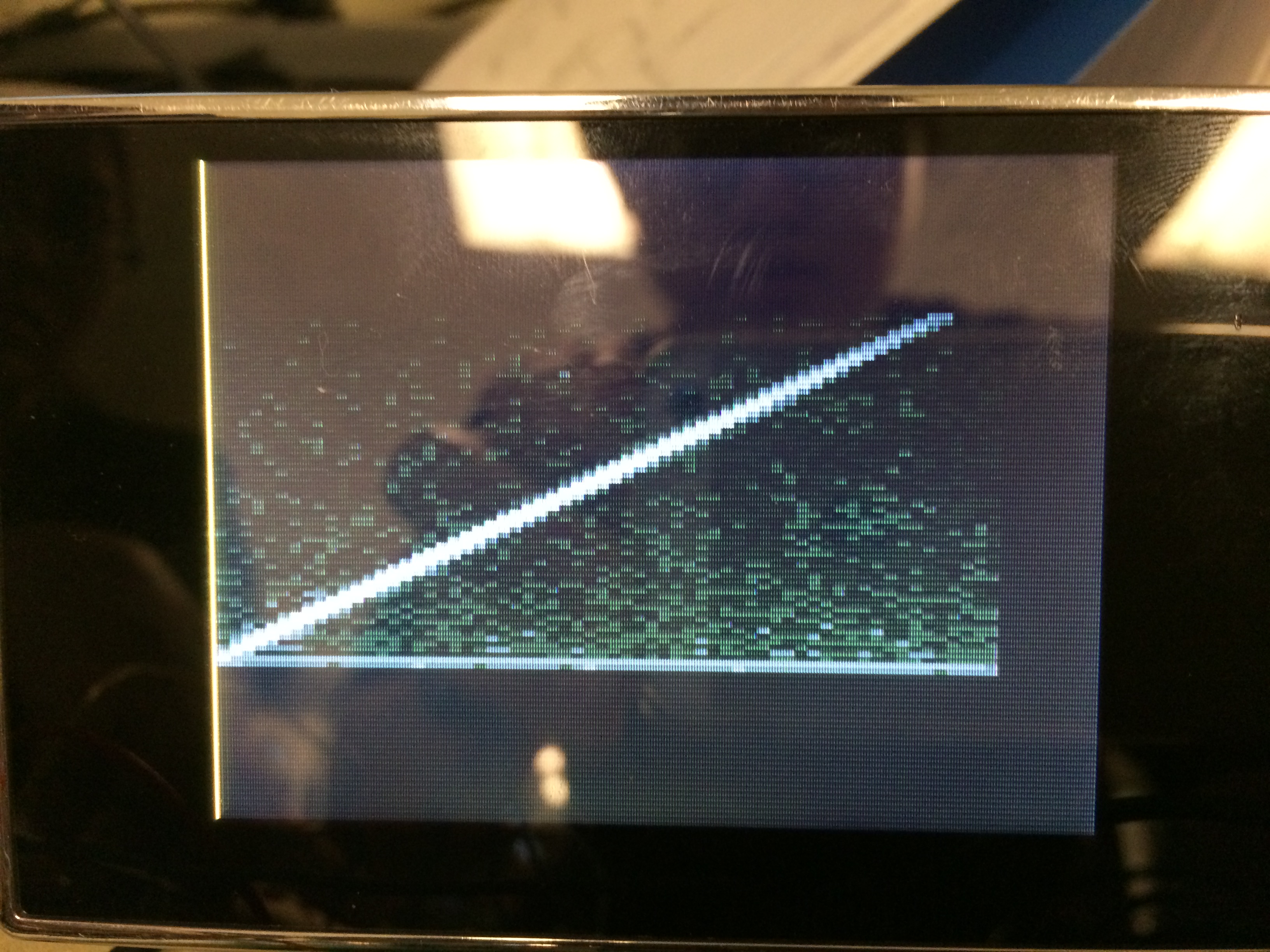
We conducted several tests to determine the temporal and frequential accuracy of our system. The response of our system to a linear frequency sweep from 10Hz to 4kHz in one second is shown below. As can be seen, the linear sweep shows that we sweep the frequency accurately from 10Hz to 4kHz (our maximum display frequency) without any distortion. We can also observe our low-pass filter being applied at 3kHz cutoff, as the signal becomes darker on the higher portion of the display.
While testing with pure sinusoids, we noticed that we have some leakage of frequency in our output, especially in the frequency bins that are just at the top and bottom of the actual frequency. As can be seen in the image below, the frequency bins adjacent to the accurate frequency bin have slightly lower - but nonzero - frequency intensities. We attribute this to several factors: first off, since we use a fixed-point FFT algorithm, there is inherent quantization error present while calculating the FFT conversion. Secondly, although we use a Hanning window to minimize frequency leakage, it cannot eliminate it completely. Thirdly, There may be errors during the ADC conversion, since during the conversion step some quantization error is introduced. In the end, we felt that this was not a huge drawback to our system since the correct frequency is still being displayed.
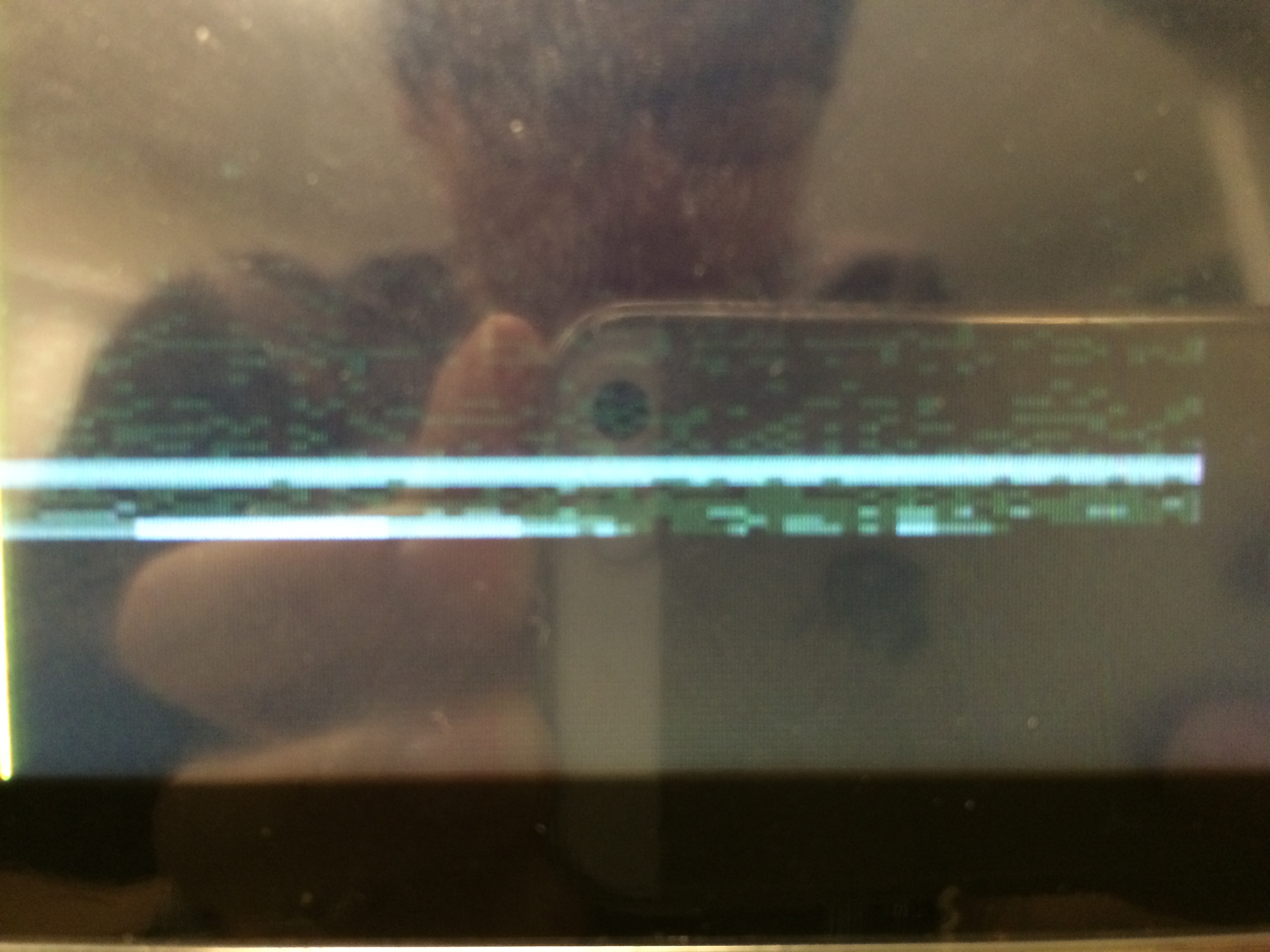
Lastly, as can be observed from the two above images there is a horizontal line across the bottom of the display. This is due to the DC-bias of the audio signal showing up as a low frequency content in our spectrogram. We considered removing this artifact by artificially nullifying the lowest frequency intensity, but we felt that the bottom line actually serves as a good indicator of where are spectrogram starts on the display, so we kept it there. Last but not least, there is always some noise present in our spectrogram, especially from the microphone input. However, this does not interfere much with observing the important content in the spectrogram.
Result from real-world audio samples
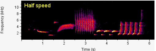
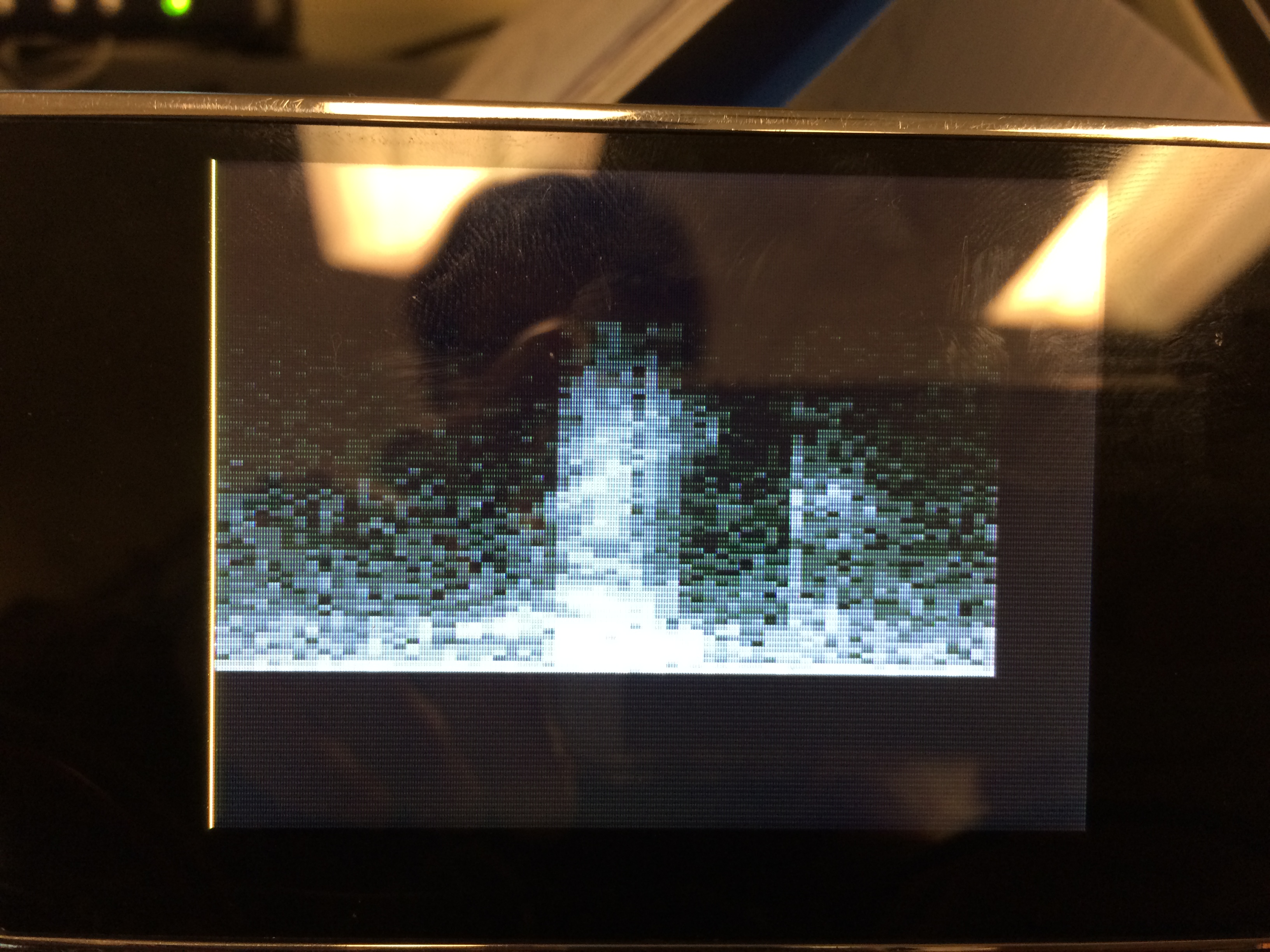
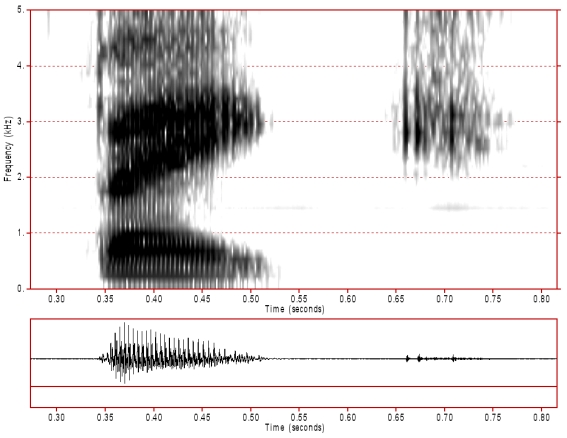
After testing several real-world audio samples, we felt the overall response of the system in terms of time, frequency, and intensity are highly accurate. Below are some spectrograms generated by our system with sample audio signals such as bird calls and human speech, with their spectrograms generated by professional programs on the side. First, we tested with a sample bird call at half speed taken from the Cornell Lab of Ornithology Website. As can be seen from the video, the spectrogram contents are almost an exact match to the spectrogram provided for us by the Ornithology Website. Note that we played the bird call at half speed, so the frequencies present in the bird calls have been reduced by half.
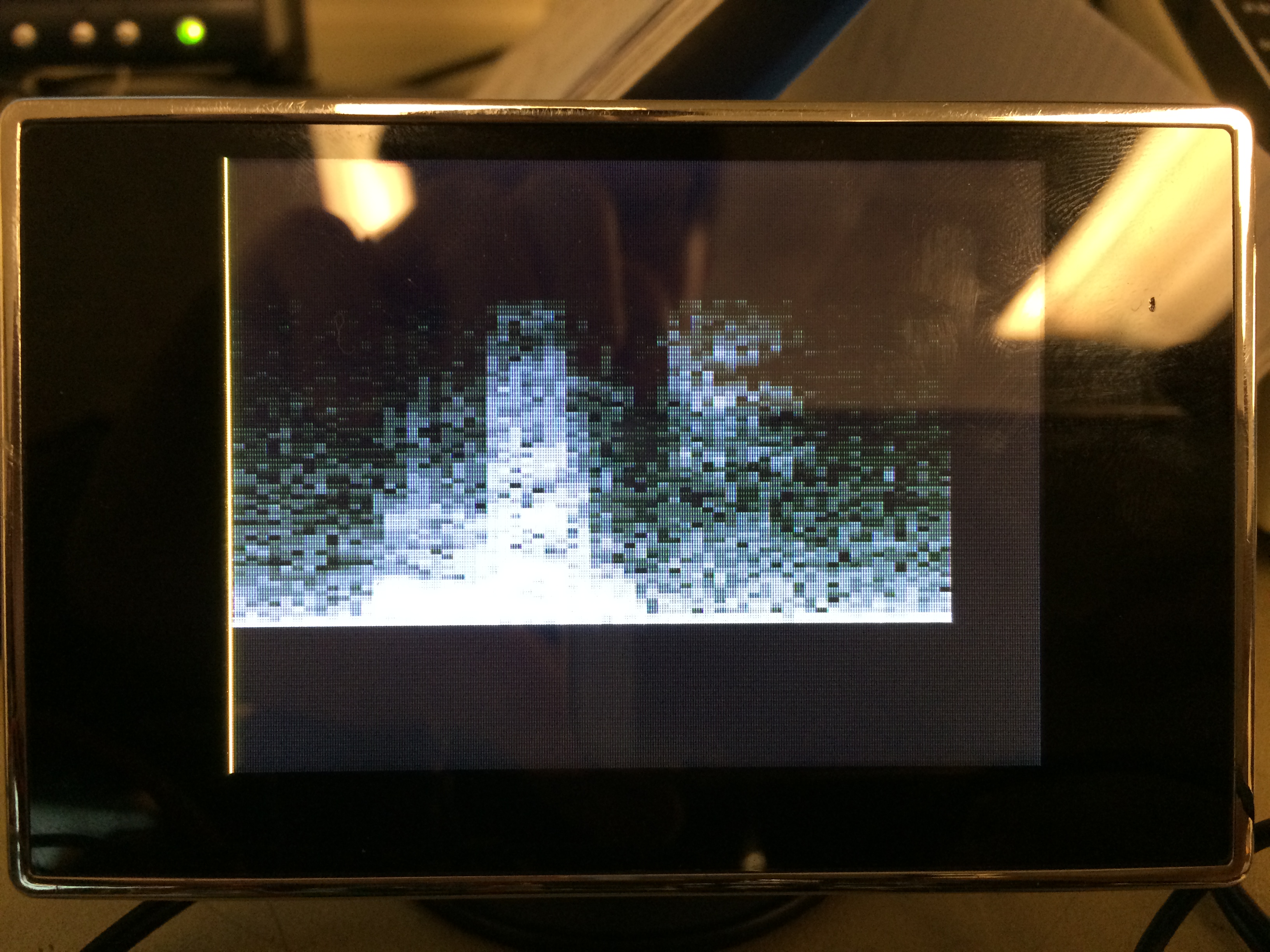
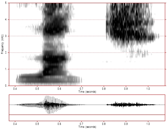
The following are the results from pronouncing the words "bake" and "lunch", and their respective paradigmatic spectrograms taken from the Consonant Spectrogram Samples page. Just like the bird calls, you can observe that the spectrograms are very similar, despite the fact that our spectrograms are much lower resolution.
Safety
There are no major safety considerations required for this project. It does not use high voltages, wireless transmission or mechanical parts. There is no direct physical interaction between the user and the device save for the push buttons, which are electrically isolated by design. The brightness of the television screen may strain the user's eye, but many televisions have brightness controls built into them, so this is not an issue.
Interference
Since we use no wireless signals, there is no worry of interference with other devices. Since our device has a microphone input, there is the reverse possibility that our spectrogram output from the microphone be interfered by the surrounding noise, which happened quite often during our demo.
Usability
Since the only interaction with the device is through the three push buttons, there are no major usability concerns. The user may have to first learn the functionality corresponding to each button since they are not labeled in any way, but since the number of buttons is small this is not a huge concern.Conclusions
Summary
The final results of the project were extremely satisfying. We were able to meet the majority of our expectations set in the project proposal. We succeeded in implementing a fully functional audio spectrogram with a scrolling display (sliding visualization) using 4-bit grayscale in real time. The project accurately displayed the frequency content with a histogram visualization of the input audio. The spectrum output from the project is aesthetically pleasing. We also were able to keep the material costs down and make it user friendly. By using standard 3.5mm audio jacks, any user with a music producing device, standard auxiliary audio and video cords, and NTSC-compatible TV could use the product. The added user options through the push button interface introduced the ability to personalize the display. As we used grayscale representation, user could see the difference in intensity levels in the audio signal. This project not only allows the users to view their favorite music in a fun and interactive fashion, but it also offers information about their music otherwise inaccessible.
Future Improvements
Future improvements that we considered implementing in the project but could not due to time-constraint include Color video output and Comparing the speech pattern (e.g. pronunciation, tempo, pitch, etc) of different users by displaying the frequency spectrum of the audio input taken on NTSC television.The color video could have enhanced the visualization by using certain color levels to indicate certain amplitude levels, and a color gradient could be implemented vertically across the bars. Since we had already implemented a 4-bit grayscale which helps to visualize the various amplitude levels in the signal using varying intensities in black and white, the color video definitely could have been implemented with some extra time.
To enable the users to vary the time scale of the scrolling spectrogram by controlling a trimpot where minimal resistance means smallest time scale and maximal resistance means the largest time scale (i.e. real time). By definition, a smaller time scale will require a delay to the signal. This implementation wouldn’t take much effort, but as for the time being we thought that this is not that critical, so we concentrated on the core part of the project.
The system will have an additional output mode controllable by the user. In this mode, a sentence will be displayed on the LCD screen. One user will first be able to record his/her reading of the sentence via the microphone. The recorded spectrogram will be displayed on the bottom half portion of the television. Afterwards, another user can read the sentence displayed on the LCD, which will be displayed on the upper half portion of the television screen in real-time. Thus, the other user can observe how similar his speech pattern is (e.g. pronunciation, tempo, pitch, etc), with respect to the recording person. This part would have been interesting if we implemented. This part definitely could have been implemented with some extra time.
More Compliance Considerations
The only standard relevant to our project was the NTSC analog television standard. We made sure that we followed and conformed to all the standards relevant to the project.
Intellectual Property
There are several intellectual property considerations regarding our project. The code to calculate the FFT was adopted from code provided by Bruce Land, which is based on code originally authored by Tom Roberts and improved by Malcolm Slaney. The video portion of our software was based on example code written in part by Shane Pryor, David Perez de la Cruz, Ed Lau, and Morgan D. Jones, all of which was modified and adapted for the Mega1284 by Bruce Land. This same section also contained portions of our own code from Lab 3 in ECE 4760 Fall 2014. Some sections of this report are also adapted from our own write up for Lab 3 of the same course and from “Audio Spectrum Analyzer” final project of Alexander Wang and Bill Jo (Fall 2012). All diagrams used are our own work or from the course website, except for the spectrograms taken from Cornell Lab of Ornithology and Macquarie University, which are used solely for demonstration purposes. All videos used in this website are our own work as well, and the bird call played is the property of Cornell Lab of Ornithology and is solely for demonstration purposes. All of the borrowed intellectual property is referenced in the References section, and borrowed due to the fact that it was provided by the course content or instructor.
Ethical Considerations
During the course of working on this final project in ECE 4760, we made sure to follow the IEEE Code of Ethics with strict accordance. We ensured that neither ours nor the user’s safety is at stake while working on the project. There are no high voltage/current sources that could hurt a person using our project. So, there are no safety measures to be taken while operating the project. We kept our lab space clean and minimal. We began the task after making sure that we have a good and attainable design that was thoroughly reviewed by us. We gave credit when using the code from the ECE 4760 website in order to prevent any perceived conflicts of interests. When stating our lists of cost estimates, we were accurate and honest, not concealing any potential costs that we know of. We were also quite self- critical of our own design, accepting honest criticism of our work to help us improve. We seeked the help of the instructor whenever we couldn’t figure out how to tackle an issue. We are not biased towards anyone based on any factors, such as race, religion, and national origins. We treated all of our peers with respect and did not say or publish anything offensive while in lab. We were respectful to others wishes and used headphones for music when possible. We cited all contributions made to the project including any of our own previous work. Overall, we honestly tried to create the best project that we could, given our time constraints, and we were honest with others and ourselves throughout the process.
Legal Considerations
There are no major legal considerations to be concerned as we did not transgress upon any intellectual property. The project does not pose any known danger to any people or property. We use standard 9-12V AC adapters to power our design, all of which should conform to legal standards.Appendices
A. Code Listing
Source code can be found at the "Extras" tab on the top-right corner of the web page.
B. Schematics
C. Budget Considerations
| Item Name | Vendor | Unit Price | Qty. | Subtotal |
|---|---|---|---|---|
| ATmega1284p | Lab Stock | $5.00 | 2 | $10.00 |
| STK500 Programmer | Lab Stock | $15.00 | 1 | $15.00 |
| 6" Prototype PCB | Lab Stock | $2.50 | 1 | $2.50 |
| Power Supply | Lab Stock | $5.00 | 2 | $10.00 |
| MCU PCB | Lab Stock | $4.00 | 2 | $8.00 |
| LCD TV | Lab Stock | $5.00 | 1 | $5.00 |
| Header Pins† | Lab Stock | $0.05 | 15 | $0.75 |
| DIP Sockets† | Lab Stock | $0.50 | 5 | $2.50 |
| MAX295 8th-order LPF* | Maxim Integrated | $0.00 | 1 | $0.00 |
| 2N3904 NPN Transistor | Lab Stock | $0.03 | 1 | $0.03 |
| Pushbutton Switch† | Lab Stock | $0.50 | 3 | $1.50 |
| Audio Jack† | Lab Stock | $0.50 | 2 | $1.00 |
| Sliding Switch† | Lab Stock | $1.00 | 1 | $1.00 |
| Microphone† | Lab Stock | $1.00 | 1 | $1.00 |
| Assorted 5% Resistors | Lab Stock | $0.30 | 32 | $9.60 |
| Assorted Capacitors | Lab Stock | $0.20 | 8 | $1.60 |
| Total Cost | $68.48 | |||
| * denotes sampled product, † denotes best estimate | ||||
D. Distribution of Work
Because it was integral for each group member to understand each separate part's operation, the development of the software and hardware was roughly shared between the three of us. Because of this, the planning and development of both the software were done with all of us present. During implementation of the developed plans, Varun worked more on the hardware than the software while Hyun Ryong and Madhuri focused a little more on the software implementation. The Specific distribution is as follows:
Varun Hegde
- Design of Audio Amplification & Filtering Hardware
- Soldering Audio Amplification & Filtering Circuit
- Web Page Design
- Hardware Schematics
Hyun Ryong Lee
- Implementing FFT Conversion and Video Generation Code
- Circular Buffer Implementation and Optimization
- Gray-scale Generation Code
- Push button State Machines
Madhuri Kandepi
- Audio Sampling and UART Transmission Code
- Design of Circular Buffer
- Gray-Scale Debugging
- Accumulating Results Data
References
Datasheets
- ATmega1284P Datasheet
- Maxim Integrated, MAX295 8th Order LPF Datasheet
- Texas Instruments, LM358 Power Operational Amplifier Datasheet
- CMB-6544PF Electret Condenser Microphone
Referenced Code
Other References
- Audio Spectrum Analyzer Project
- Wikipedia: Voice Frequency
- Frequencies of Musical Notes
- Stanford EE 281 Laboratory Assignment #4: "TV Paint"
- Frequencies of Musical Notes
- Cornell Lab of Ornithology - What is a Sound Spectrogram?
- Macquarie University - Sample Single Syllable Spectrograms