Program/Hardware Design

 

Hardware Design

 

Since the output of the guitar will be at low amplitude (about 3mV peek to peek), we must amplify the signal before running it to the Mega32’s ADC. To do this, we used the circuit shown below:

 

 

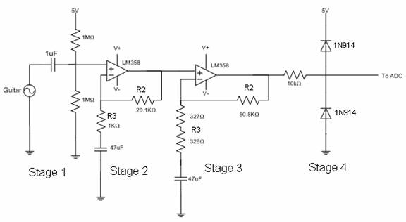
Fig. 3: This is a schematic of the analog circuitry used to amplify the guitar output before it enters the ADC. Each stage is described below.

 

 

 

Stage 1

 

The purpose of stage 1 is to filter out any DC bias the guitar may be applying to its AC output. We attached the guitar using alligator clips from the plug of the cable to the input and ground. The 1uF capacitor effectively blocks any DC bias and the two 1M-ohm resistors introduce a 2.5V bias to the AC signal to center it. In actuality, the bias introduced depended on the power source we were using. Variances were usually in the plus or minus 50mV range. These variances didn’t affect our software in any significant way because software was able to compensate for the variance. It is important to note the 3DB frequency (half amplitude) of the filter created by the 1uF capacitor and 1M-ohm resistor. The frequency of this high-pass filter is given by f = 1/(2*pi*R3*C) = 0.16 Hz.

 

Stage 2

 

The purpose of this stage is to amplify the guitar signal but block DC amplification. Since the DC offset is 2.5V, amplifying the bias would cause the opamp to rail. For this reason, we put in a capacitor to ground, effectively blocking DC amplification. The low pass filter to ground formed by the capacitor and resistor has a 3DB cutoff frequency of f = 1/(2*pi*R3*C) = 3.39 Hz. The opamp is set up in a non-inverting amplifier configuration, which has a voltage gain of Av = 1 + R2/R3 = 1 + 20.1/1 = 21.1. The values of V+ and V- will be discussed in stage 3 because they are defined by the necessities of that stage.

 

Stage 3

 

Stage 3 is very similar to stage 2. Its purpose is to further amplify the signal so that it gets into the 5V to 0V range (2.5V peek to peek with a 2.5V bias). This amplifier has a gain of Av = 1 + R2/R3 where R2 is the series combination of the 327-ohm and 328-ohm resistors (655 -ohms). Thus Av = 77.5. The total gain from stages 2 and 3 is thus 21.1 * 77.5 = 1636, yeilding a peek to peek voltage of 3mV * 1636 = 4.9V. Its important to note here that the values of V+ and V- are arbitrary as long as they exceed roughly 5.5V and -5.5V, respectively. We need these to be the rails of the op-amp to prevent clipping at roughly 4.5V (because the LM358 looses a diode-drop's worth of voltage). By increasing the rails of the opamp, we were able to amplify the AC into the 5V to 0V rails. This was done by trial and error: we turned the knobs on the voltage source until we saw no clipping on the oscilloscope. The low pass filter to ground formed by the capacitor and resistor has a 3DB cutoff frequency of f = 1/(2*pi*R3*C) = 5.13Hz. Thus, overall, the circuit cuts out any frequencies below 5.13Hz. This isn’t a problem because this low frequency is out of the range of human hearing and unachievable on the guitar.

 

Stage 4

 

The purpose of this stage was to limit the voltage seen by the MCU. Since we didn't want to overload the ADC port, we needed to limit the voltage seen by ADC to within one diode drop of 5V or 0V. This is why we used the two diodes with the 10k resistor. The MCU's input port resistance dwarfs this 10k resistor but it provides a place to dissipate any power going to 5V or 0V through either diode. Without this 10k resistance one of the diodes would dissipate the power, probably burning it out.

 

 

Program Design

 

We used an interrupt driven task scheduler to implement our tuner. We set timer.0 to interrupt every 0.2 ms and used the interrupt to drive two tasks: sample() and buttonSM().

 

The task buttonSM() is run every 0.2 ms. It samples and filters the input from the ADC, measures the length of ten periods and compares it with a target period for the string being tuned. If the measured period is less than the target period the program sets the LEDs indicating that the string’s frequency is too high. If it is greater than the target period the programs sets the LEDs indicated that the string’s frequency is too low. If it is within a predetermined bound from the target the ‘in tune’ LED is lit.

 

Fig. 4: The box represents the program flow when task sample() is run. Because the task is run every 0.2 ms the signal x(t) is sampled at 5 kHz.

 

 

The user determines which string is being tuned by pressing one of 6 buttons where each button corresponds to a string. The task buttonSM() is run every 30 ms and detects the button presses. It then sets the state variable ‘string’ to the value corresponding to the pressed button and runs set_string(). The task set_string() outputs the name of the string being tuned to the LCD and sets all the period bounds and filter coefficients based on the values stored in arrays.

 

During initialization, three different levels of bounds on the period are determined for each string. The largest bounds set the limit on triggering. No triggering or period measurements will be made wile the input frequency is outside these largest bounds. The smallest bounds determine if the string is in tune. Along as the input frequency is within the tight bounds than it is within 0.5% of the desired frequency and the string is considered to be in tune. The medium sized bounds are in between and determine which LEDs are lit. The largest bounds are created by multiplying and dividing the target period by a factor that corresponds to roughly a whole step. The notes that we here are related to the frequency by the following equation:

 

 

In the equation, ‘C0’is the frequency of the note C0 and ‘n’ is the number of semitones above C0. It is easy to see that by multiplying or dividing the target frequency by 2^(1/12) creates frequency bounds that corresponds to plus or minus one semitone.

 

Filtering

 

To calculate the period of the input signal we counted the number of samples between zero-crossings. Zero-crossings occur when the input signal goes from below to above a bias voltage centered in the middle of the signals voltage range. All of the guitar strings contain higher harmonics and the second harmonics are large enough that they may cause additional zero-crossings to the input signal. Therefore, if the higher harmonics are not removed through filtering, then a true measurement of the period can not be obtained.

 

In choosing a filtering method we needed to trade off between ideal filter characteristics and speed of filtering. Since the second harmonics are always twice the fundamental frequency, the filter did not need to have a steep cutoff. Also, because the device was limited by how many calculations could be performed the filter needed to be vary fast. Therefore, we used a simple low-pass infinite impulse response (IIR) filter to remove the higher harmonics. The filter does not have a very steep cutoff but is very fast to implement because it requires only two multiplies and one divide which can be implemented via a shift. For an input signal x(n) and a filtered signal y(n) the filtering is performed with the following equation:

 

 

In the equation ‘a’ is a parameter between zero and one which determines the width of the low pass filter. If ‘a’ is near zero the filter is similar to an all-pass filter and very little filtering is done. If ‘a’ is near one the filter has a very steep cutoff and only very low frequencies will be retained. To see this, observe that the frequency response of the filter is given below where T is the sampling period of 0.2 ms:

 

 

 

Because the denominator increases with frequency (until the frequency reaches half of the sampling frequency) this filter acts as a low pas filter. To filter the guitar strings such that only the fundamental frequency induced zero-crossings, we had to make sure that the second harmonic was greatly attenuated with respect to the first harmonic. However, we could not make ‘a’ too large or we would not be able to detect the fundamental frequency. Therefore the program sets the value of ‘a’ depending on which string is being tuned. Larger values are used for the low strings and smaller values for the high strings. Below are two graphs, one in the time domain and one in the frequency domain, showing the unfiltered and filtered samples of the b-string. Notice that filter H is shown in the second graph.

Fig. 5: This is a 16 ms segment of the input from ADC. Notice that the secondary humps in the unfiltered signal cause zero-crossings. Also, the amplitude of the filtered signal is much less than the unfiltered signal.

 

 

 

Fig. 6: These are the DFTs of the filtered and unfiltered 16 ms segment of the input from ADC along with the frequency response (Discrete Time Fourier Transform) of the filter. Notice that the second harmonic is attenuated by a factor of 0.2 while the first harmonic is attenuated by a factor of 0.55.

 

 

Things We Tried That Didn't Work

 

Hardware

At first we thought we could achieve the high gain necessary using only one op-amp. This proved to be impractical because the output fluctuated substantially and was somewhat noisy. After we moved to the two op-amp scheme, we found that the gain on stage 3 was very sensitive. We knew we wanted a gain of roughly 1666 (5V/3mV) but we had to try a lot of different resistor combinations for both R2 and R3 (of both stage 2 and 3) until we found one that was suitable. In retrospect, it may have been more efficient to use a potentiometer for either R2 or R3 or both.

 

Program

Initially we measured the input frequency by measuring the length of only one period. This was a very poor idea because the period of the high e corresponds to only 15 samples. This meant we had very poor accuracy when trying to determine the true period of the input. To add some accuracy we tried to interpolate a straight line between the points on both sides of the zero-crossings. This involved two add operations and one divide. This technique added some accuracy but was still very unreliable when the input signal was not a nice sine wave. We therefore ended up counting ten periods instead of one to achieve necessary accuracy and stability. 

 

 

Filtering

When we first looked at the input signals from the guitar we thought that perhaps we would not need to do any filtering because the input signals had spikes that coincided with their fundamental frequencies. We reasoned that if we simply moved the bias up to the point that only the spikes would cause triggering then we would not need to worry about the smaller humps caused by the higher harmonics. However, although the signals appeared nice over small time spans their form fluctuated over longer time spans. As the string rang, the orientation and size of the secondary humps changed such that there was never a bias which would always trigger on only the fundamental frequency.

 

 

Testing

 

Since we couldn't always bring the guitar to lab (and we had to test the accuracy and amplification of the circuit) we had to use the signal generator to fake the guitar input. The way we did this was rather tricky. Even when the amplitude of the signal generator was turned all the way down the amplitude was still about 50mV peek to peek (remember we needed to get down to 3mV peek to peek to fake the guitar signal amplitude). Thus, we ran the signal generator output through a potentiometer, which we tuned until we got a 3mV peek to peek signal. It was difficult to determine the exact amplitude because the oscilloscope couldn't cut through the huge amount of noise coming out of the signal generator. We had to "eyeball" the amplitude from the oscilloscope screen. Surprisingly, the guitar was a much better signal generator than the one in the lab. The guitar input was significantly less noisy, although the hardware cut out all the noise (even from the signal generator) before routing the signal to the ADC. 

 

We tested the accuracy of the device by tuning the guitar until the middle LED was lit, which meant the device read the input as being in-tune. To assure accuracy, we plugged the guitar into a handheld guitar tuner and saw that that the input was usually a few percent below what it should have been. We calibrated the device accordingly and re-tested until we match the handheld guitar tuner’s assessment.