Cornell University ECE4760
FIR filter designer
Pi Pico RP2040

FIR filters in s1x14 fixed point with downsampler, and window design commands.

This project constructs a finite-impulse response (FIR) filter designer using window design methods. The user specifies a filter type (lowpass, bandpass, highpass), the relevant frequencies, a filter length (up to about 60 at 40KHz), and a window-type. The supported window-types are rectangular, Hamming, and Blackman. Rectangular has the fastest rolloff, but terrible stop-band attenuation of -20 db. Hamming has reasonable rolloff and good stop-band attenuation. Blackman has slower rolloff, but best stop-band attenuation. No matter what you do, with 14 bit coefficients, the best attenuation you can relably get is -67 db, or for unity input amplitude about 4x10^-4 output amplitude.

The actual filtering is done in an ISR running at 40 KHz, so we are designing audio-rate filters. The arithmetic is fixed point s1x14 format (16-bit total: a sign bit, one integer bit, 14 fractional bits). After designing a filter, the program may be set to do realtime filtering of audio signals using the ADC channel zero input. Actual filter input and output are displayed using a SPI DAC.

FIR filters take about 10 times the compuation to reach the same cutoff bandwidth as IIR filters. The ONLY andvantages to FIR filters are: (1) linear phase in the passband, which means good pulse response, and (2) the filter frequency response is complicated, such as HRIR for localizing sounds. If you are trying to detect a given frequency, building an audio equalizer, or speech vocoder, use IIR filters. Fixed point s1x14 format filters are about 15 times faster to execute than floating point, about 4 filter taps per uSec, but are still slower than IIR filters.

For low frequency filters you will need to downsample, so that the ratio of bandwith to Nyquist rate is not too small. A CIC filter is used to drop the sample rate by 4, while avoiding aliasing.

All filters implement the "Direct Form II " implementation of a difference equation shown below (from the Matlab or Octave filter description), where nb is the filter-length. The y(n) term is the current filter output and x(n) is the current filter input. The and b's are constant coefficients, determined by some design process. Here we are using a window algorithm, but you could get coefficients in Python, Octave, or Matlab.

    y(n) = b(0)*x(n) + b(1)*x(n-1) + ... + b(nb)*x(n-nb)   

All program functions are controlled by a simple command sequence.

• lp cutoff_freq filter_length window_type
  The lp command takes three parameters: the cutoff frequency in Hz.
  The filter length, which can vary from 10 to 60 at 40 KHz sample rate.
  The window used to smooth the impulse response. Values are r, h, b for rect, Hamming, Blackman.
  
• hp cutoff_freq filter_length window_type
  Parameters have the same meaning as above.
• bp low_freq high_freq filter_length window_type
  The low frequency is the low band edge frequency of the bandpass. LIkewise high frequency.
• boxcar filter_length
  This is a very crude running average filter with no windowing.
  The effective stop-band edge is given by the filter-length.
  I used it for calibration. Dont use it in production.
  --- display controls ---
• freq low high increment
  Control the plotting frequency range.
  On the default log plot you set from low to high with ratio increment (>1, typically 1.02 to 2)
  On the linear plot you set from low to high with increment ( typically 50 to 500).
• color single_letter
  One of: g, r, b, c, m, w, y for the plot (green, red, blue, cyan, magenta, white, yellow),
  The chosen color will be used for the next Bode plot.
• downsample yes/no
  A yes performs a 4x sample slowdown before the filter. This shifts the filter frequencies lower.
• erase
  clears plot, draws axes
• dac yes/no
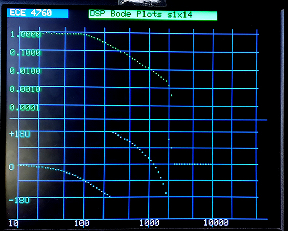
  A yes turns on a two channel SPI DAC displaying the filter input and output. The DAC is also turned on by the realtime command below.
• realtime yes/no
  A yes turns on channel zero of the ADC and applies it to the filter you just designed.
  Designing a new filter while realtime is turned on automatically turns it off!
  

On the first plots, frequency grid lines are logarithmic, with decade, 2's (e.g. 20,200,200) and 5's (e.g. 50, 500, 5000) drawn. Amplitude in the upper plot is logarithmic, with decade lines drawn and labeled. Phase in the lower plot is a linear scale. At low frequency there may be some noise in the plot because the averaging time of the cross-correlation used to get the phase and magnitude did not average enough samples. To get phase and magnitude, the filter output was cross-correlated with the filter input sine wave, and a 90-degree phased shifted version of the sine wave. These are refered to as the I (in-phase) and Q (quatrature) channels of the correlation. You can think of the I and Q signals as the vector components of the output voltage. The average value of the magnitude of the vector is the output amplitide and the arctan of the ratio of the average of I and Q is the phase.

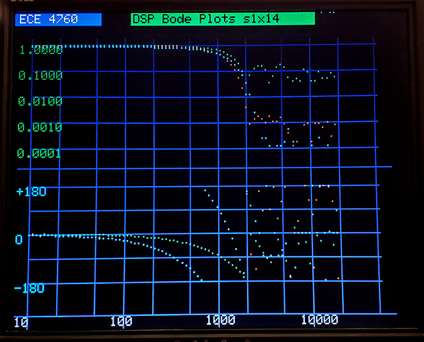
The lowpass below shows boxcar 20 (green), lp 1000 60 h (red), lp 1000 60 b (cyan). You can see that the Hamming and Blackman windowed designs with 60 taps bottom out at around 5e-4, in line with accuracy estimates. Hamming has a little faster rolloff. The boxcar has low stop-band attenuation.

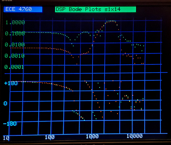
A bandpass filter with low band-edge at 2000 and high band-edge at 4000, with 60 taps. Green is rectangular window, red is Hamming window.

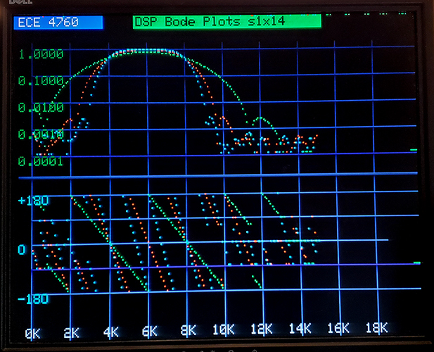
A possibly more familiar plot of the bandpass function is shown below on a linear-frequency plot. The linear-phase nature of the FIR response is much more obvious, as are the symmetrical low and high frequency rolloffs. The commands below were used to generate 20, 40 and 60 tap filters with Hamming window. You can see that the band edges get steeper with increasing tap number.
filter cmd> erase
filter cmd> freq 100 15000 100
filter cmd> color r
filter cmd> bp 4000 8000 40 h
filter cmd> color g
filter cmd> bp 4000 8000 20 h
filter cmd> color c
filter cmd> bp 4000 8000 60 h

The program is bulky because it handles the graphics to plot the frequency responses, supports a command language, computes the filter coeffients from user specifications, specifies several filter types, and runs a 40 KHz ISR to actually do the filtering. This ISR sweeps a frequency over the desired range using DDS, runs the desired digital filter using the DDS as input, then computes the cross-correlation of the filter output with the DDS input, and with a second DDS signal which is in quadrature with the filter input. From the average correlations, the graphics thread computes the Bode plots of filter phase and magnitude. The phase/magnitude calculations become inaccurate at very low frequency, or low filter output amplitude. You can see that in the bandpass plots above.

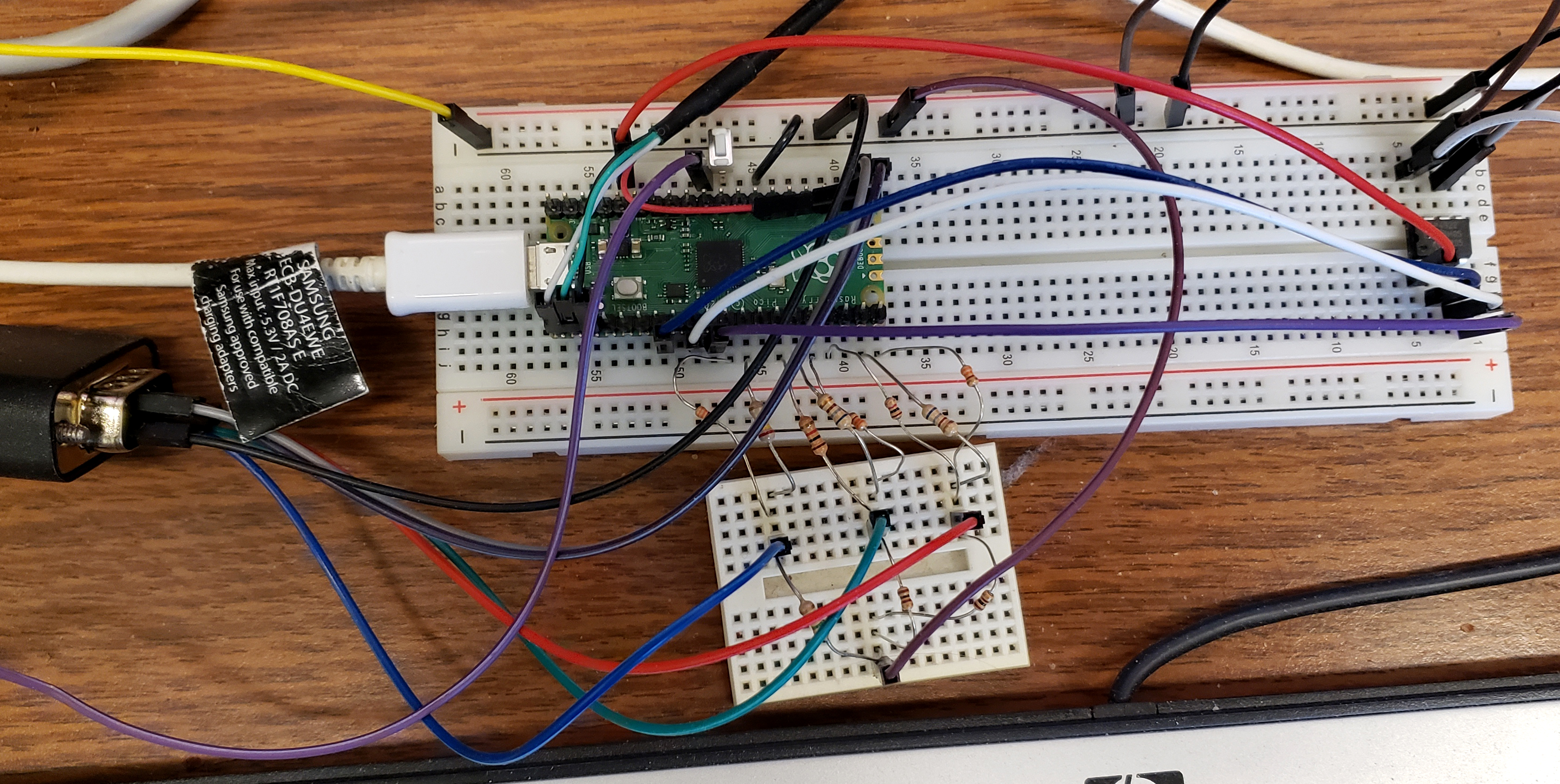
For everything to work, you need to attach a VGA monitor, a MCP4822 SPI DAC, and a signal source to ADC channel zero (source voltage must be between zero and Vdd volts). More hardware details are also in the code.
Photo of circuit.

Code, project ZIP, Mod for linear plot

CIC downsampler.
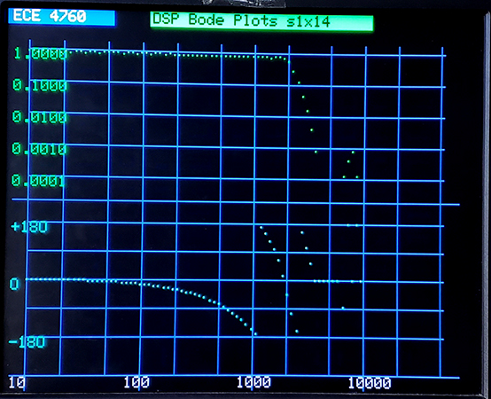
Narrow bandwidth FIRs get harder at low frequency. With the full sample rate of 40KHz (Nyquist rate 20KHz), then downsampling by 4, the Nyquist rate is 5KHz. The 4th order CIC filter, plus Chebshev compensator has a rapid cutoff at 2 KHz, or 0.4 normalized to the new Nyquist rate. The first image below is the downsampler Bode plot. Note the fast cutoff at 2KHz, dropping to below 0.001 amplitude before the 5KHz Nyquest rate. The second plot is a Butterworth 2-pole lowpass feed by the downsampler. The cutoff of the lowpass is 0.025 of the downsampled Nyquist rate.

Copyright Cornell University June 9, 2023