Floating Point DDA on FPGA
A modern Analog-style Computer
The Digital Differential Analyzer (DDA) is a device to directly compute the solution of differential equations. The DDA is a simulation of an analog computer, and is inherently parallel in operation. It can be mapped easily into an FPGA by defining mathematical integrators, adders, multipliers and other operations, then wiring them together to produce the desired dynamics.
For more background on analog computers see:
The general approach using DDAs will be to simulate a system of first-order differential equations, which can be nonlinear.
Analog computers use operational amplifiers to do mathematical integration.
We will use digital summers and registers. For any set of differential equations with state variables v1 to vm:
dv1/dt = f1(t,v1,v2,v3,...vm)

dv2/dt = f2(t,v1,v2,v3,...vm)

dv3/dt = f3(t,v1,v2,v3,...vm)
...
dvm/dt = fm(...)
We will build the following circuitry to perform an Euler integration approximation to these equations in the form
v1(n+1) = v1(n) + dt*(f1(t,v1(n),v2(n),v3(n),...vm(n))

v2(n+1) = v2(n) + dt*(f2(t,v1(n),v2(n),v3(n),...vm(n))

v3(n+1) = v3(n) + dt*(f3(t,v1(n),v2(n),v3(n),...vm(n))

...

vm(n+1) = vm(n) + dt*(fm(...))
Where the variable values at time step n are updated to form the values at time step n+1. Each equation will require one Euler integrator.
The multiply may be replaced by a shift-right if dt is chosen to be a power of two. Most of the design complexity will be in calculating F(t,V(n)). V(n) is a vector of all the state variables. Later we will replace this with a more stable integrator.

We also need a number representation. I chose 18-bit mantissa, 8-bit exponent floating point format written by Mark Eiding and modified for Cyclone5 by me.
- Functions:
- floating add (pipelined, combinatorial)
- floating multiply -- combinatorial
- reciprocal square root (5-stage pipeline)
- negate -- invert the sign bit
- absolute value -- zero the sign bit
- shift -- just increment/decrement the exponent (but watch out for exponent==0)
- integer-to-float, float-to-integer conversion -- 16-bit integer conversion
- Format:
bit 26: Sign (0: pos, 1: neg)

      bits[25:18]: Exponent (unsigned)

      bits[17:0]:  Fraction (unsigned)

      (-1)^SIGN * 2^(EXP-127) * (1+.FRAC)
- Since denorms are not allowed, the high order bit in the fraction is
always 1, and does not need to be stored.
- Example:
-25.0

    ((-1)**1) * (1.100100000000000000) * (2**(131-127))

    -1     *      1.5625            *      16

    1 10000011 100100000000000000 (Note that the integer part of 1.1001 is not actually stored)

    0x60E4000
- If the exponent is zero then the value should be treated as zero independent of the mantissa
A few numbers are shown in the table below.
Decimal number |
27-bit floating
representation
|
| 2.0 |
27'h2000000 |
1.0 |
27'h1fc0000 |
0.5 |
27'h1f80000 |
0 |
27'h0000000 |
-0.5 |
27'h5f80000 |
-1.0 |
27'h5fc0000 |
-2.0 |
27'h6000000 |
Second order system (damped spring-mass oscillator):
As an example, consider the linear, second-order differential equation resulting from a damped spring-mass system:
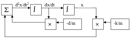
d2x/dt2 = -k/m*x-d/m*(dx/dt)
where k is the spring constant, d the damping coefficient, m the mass, and x the displacement. We will simulate this by converting the second-order system into a coupled first-order system. If we let v1=x and v2=dx/dt then the second order equation is equivalent to
dv1/dt = v2

  dv2/dt = -k/m*v1-d/m*v2
These equations can be solved by wiring together two integrators, two multipliers and an adder as shown below. In the past this would have been done by using operational amplifiers to compute each mathematical operation. Each integrator must be supplied with an initial condition. The first pass of the
Converting this diagram to run on the Cyclone5 requires control from the HPS, working along with the parallel solver on the FPGA side. In this first example, the HPS is setting up the constants, controlling reset, and controlling the analog_clock for each sample. One each sample clock, the solution is advanced one dt time-step by the parallel solver. The state of the system is maintained by the registers in the floating point integrators, while the rest of the modules are combinatorial. As seen below, the Euler method integrator uses a floating point shifter and an adder, for total size of about 550 ALMs. During testing a bug was found in the floating point shifter. The original version attempted to shift a zero value with unpredictable results.
////////////////////////////////////////////////
//// FP Euler integrator ///////////////////////
////////////////////////////////////////////////
module fp_integrator(out,funct,InitialOut,dt,clk,reset);
output [26:0] out; //the state variable V
input [26:0] funct; //the dV/dt function
input [7:0] dt ; // in units of SHIFT-right
input clk, reset; // reset high
input [26:0] InitialOut; //the initial state variable V
wire [26:0] out, funct_x_dt, new_v1 ;
reg [26:0] v1 ;
always @ (posedge clk)
begin
if (reset==1) //reset
v1 <= InitialOut ; //
else
v1 <= new_v1 ;
end
// v1 = v1 + (funct>>dt)
FpShift times_dt(funct, dt, funct_x_dt);
FpAdd_c integrator_sum(v1, funct_x_dt, new_v1);
//
assign out = v1 ;
endmodule
//////////////////////////////////////////////////
With an integrator, we can now code the two differential equations representing the factored second-order system above as
// form funct2 = (-v1xK_M -v2xD_M)
FpMul k_m(k_over_m, v1, k_m_x_v1);
FpMul d_m(d_over_m, v2, d_m_x_v2);
FpAdd_c fu2(k_m_x_v1, d_m_x_v2, funct2);
// wire the intergrators
// initial conditions of 1.0 and zero.
// dt is 2^(-9)
// module fp_integrator(out,input_funct,InitialOut,dt,clk,reset);
fp_integrator int1(v1, v2, 27'h1fc0000, 8'd9, Analog_Clock, Analog_reset);
fp_integrator int2(v2, funct2, 27'h0, 8'd9, Analog_Clock, Analog_reset);
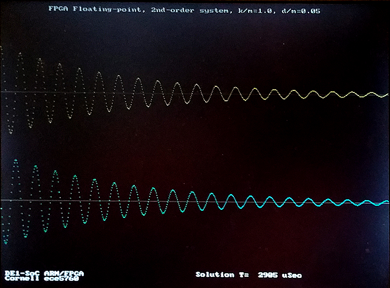
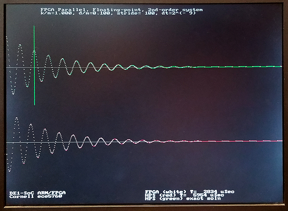
Time scaling the solution requires consideration of the value of dt and the analog_clock rate. If the time step, dt=2-9, then 29 steps must equal one time unit. For the damped spring-mass oscillator with a k/m=1.0, the solution advances one radian for every time unit (review the math). One cycle should therefore take 6.28*29 = 3215 solution steps. In the image below, the solution is ploted every 100 time steps, so there should be 32 points/cycle (there is). To get the actual frequency of the wave, you need to know how fast the solver is running. Currently the solver is running at about 22 time steps per microsecond on the FPGA, so the real period of the output sinewave is 3215/22=146 microseconds, or about 6800 Hz. The frequency (again: review mechanics) scales as sqrt(k/m). The top trace is the position, v1, and the bottom trace is the speed, v2 in the differential equations above.
The design here is hard-coded with constants, dt, and solution stride. The solution stride is defined as the number of solver steps between sending data to the HPS for plotting. The hard-coded constants are two floats and a 12-bit integer. The k/m and d/m are negated to save operations in the solution. 100 solution steps are performed between each point plotted by the HPS. The solution steps are performed with two-cycle timing, so the observed performance of 22Msamples/sec is just slightly slower than the max possible of 25Msamples/sec at 50MHz clock rate.
wire [26:0] k_over_m = 27'h5fc0000 ; // -1.0
wire [26:0] d_over_m = 27'h5ea6666 ; // -0.05
reg [11:0] stride=100;
reg [7:0] dt = 8'd9 ;
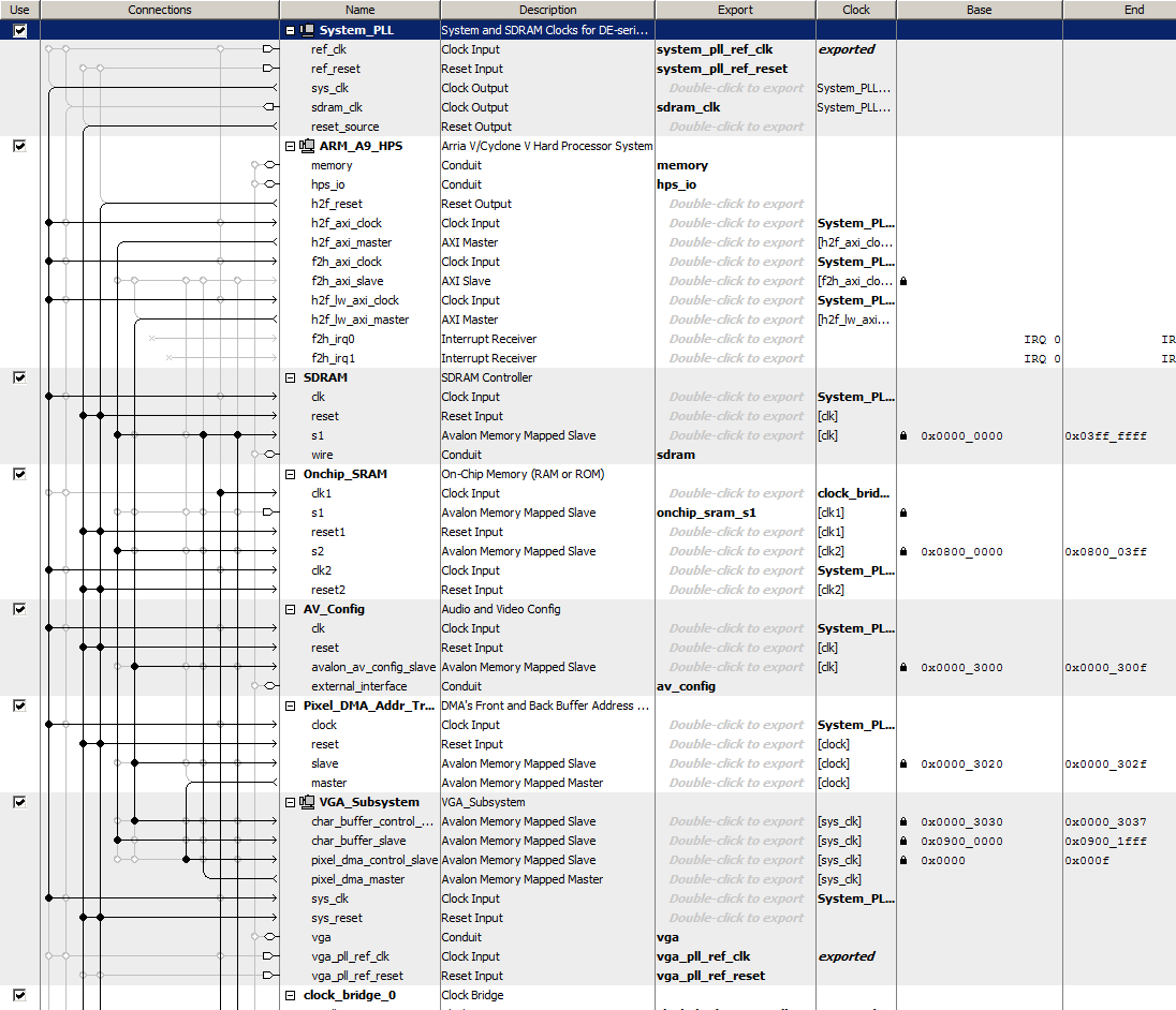
(address_header, HPS_code, top_level_verilog, ZIP_of_project) The Qsys layout is the same as the
VGA display using a bus_master as a GPU for the HPS. Display from SDRAM on the Qsys bus Master page.
The second order system solver design uses 4102 ALMs, 3798 registers and 8 DSPs. Most of this hardware is used to run the Qsys interconnect fabric.
Second order system, Euler integrator, with parameter control and compare to HPS solution
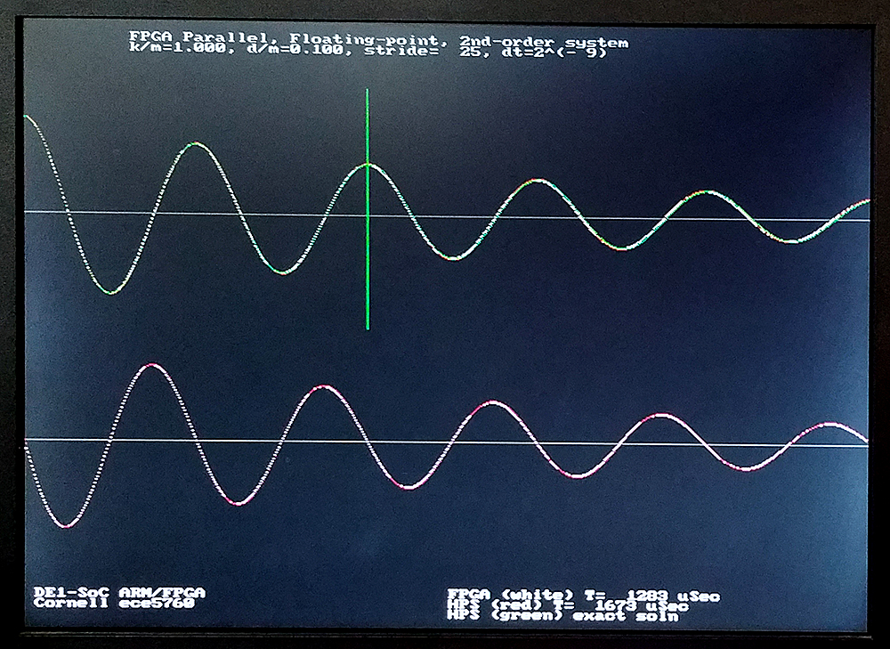
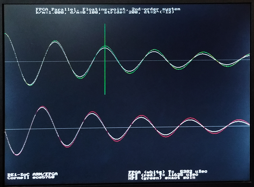
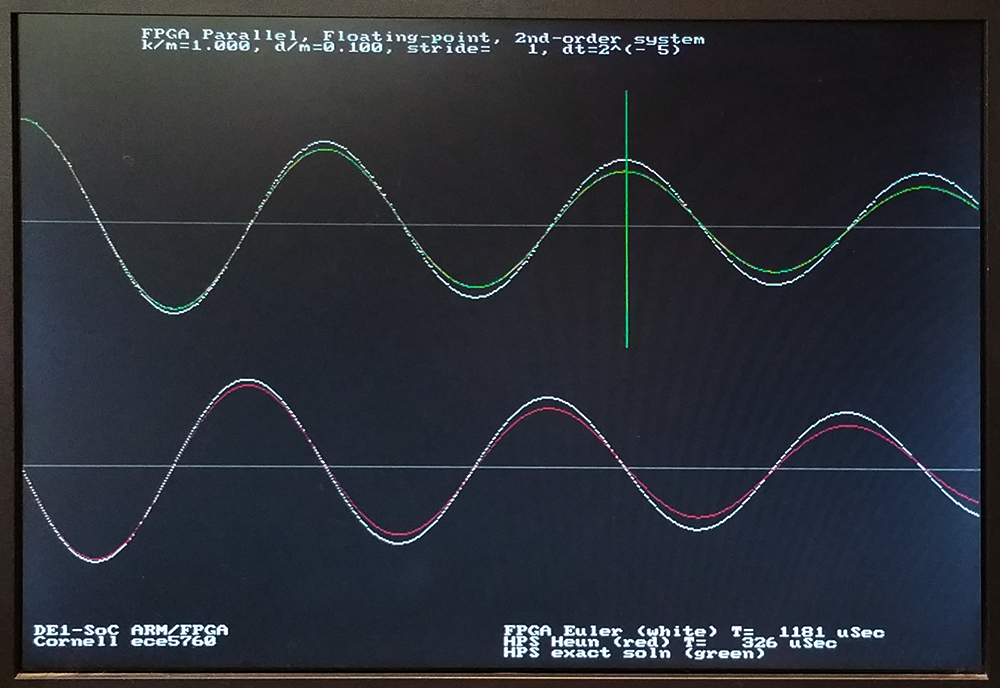
The system was modifed to load k/m, d/m, dt, and stride from the HPS command line to the solver, solve the system on the FPGA, then again on the HPS, with accuracy and time comparison. The analytical solution is plotted in green. The FPGA solutions are in white, the HPS in red on the plot below. The vertical green line should mark exactly two cycles since beginning the solution. Using a dt=2-9, all three solutions match fairly well. Relative speed of the FPGA solution changes with stride, because of read-out overhead. In the first image, the stride shown is 25, the FPGA solution is about 25% faster. For a stride of 200 second image), the FPGA is twice as fast as the HPS solution. At the dt=2-12 shown, the gain of the simulated solutions is a little low for both the FPGA and HPS. The third image shows a dt=2-9, with reasonable accuracy, and good performance. The second order system Euler solver, with parameter setting, uses 5167 ALMs, 3889 registers and 8 DSPs. Again, most of this hardware is used to run the Qsys interconnect fabric.
(HPS_code, top_level_verilog)
Second order system, Heun's Method integrator, with parameter control and compare to HPS solution
The simple Euler integrator above does not provide good accuracy with high d/m damping ratios, or for a wide range of dt. An improved Euler integrator (Heun's method) with better convergence was written. While Euler increases accuracy linearly with decreasing step size, Heun increases quadratically. The general procedure is:
- Form the slope for each variable at time=n
kv1 = f1(v1(n), v2(n)) -- dv1/dt = f1 = v2
kv2 = f2(v1(n), v2(n)) -- dv2/dt = f2 = -k/m*v1 -d/m*v2
- Estimate one step forward for each variable by Euler integration
v1t = v1 + dt*kv1
v2t = v2 + dt*kv2
- Form the slope for each variable at time=n+1 using the estimated variables
mv1 = f1(v1t, v2t) -- dv1/dt = f1 = v2t
mv2 = f2(v1t, v2t) -- dv2/dt = f2 = -k/m*v1t -d/m*v2t
- Average the two slope estimates and step forward to get the new values of V.
v1(n+1) = v1(n) + dt*(kv1 + mv1)/2
v2(n+1) = v2(n) + dt*(kv2 + mv2)/2
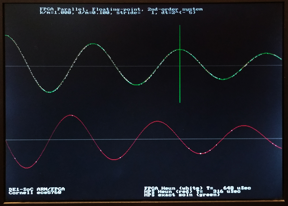
The first step is to validate Heun's Method on the HPS. The above procedure was coded and compared to Euler running on FPGA and the analytical solution running on the HPS. The image below shows a dt=2-5. The red and green curves are essentially identical, so Heun is as good as the exact solution with only 32 points/radian. Heun works fairly well down to 8 points/radian (dt=2-3), where Euler diverges (with this d/m=0.1). At small dt, Heun matches the exact solution to at least dt=2-13, while the Euler method has too low gain, particularly at high damping. At very low damping, the Euler solution diverges for dt bigger than dt=2-8.
For the Heun Method hardware implementation we need:
- Compute each slope f1, f2 at time n
-- For time=n use f1, f2 operations to form kv1 and kv2
- An adder/scale module (vnt) to compute v1t, v2t (and pipeline vnt and kvn)
-- Used to compute the next step.
- Compute each slope f1, f2 at time n+1 using the Euler approx in step 2
--For time=n+1 use the f1, f2 operations to form mv1 and mv2
- An Euler integrator to compute final values v1(n+1), v2(n+1)
-- with function input
kv1+mv1 or kv2+mv2
--
dt(huen)=dt(euler)+1 to shift it, to form dt/2
The extra operations necessary to do the two-step update drops the maximum solution rate to 12.5 million steps/sec, but with the extra wait-states, it is possible to fold the output to the HPS into the solution so that there is only a small stride-length related delay. The dt step size can be increased from dt=2-9 to perhaps dt=2-4. The solution therefore has perhaps 16-32 times fewer steps, but each step takes twice as long as for Euler integration. We thus gain FPGA execution speed by about a factor of 20 or so, with better accuracy! The execution time of the HPS code to plot the solution completely dominates the computation time. The images below use similar parameters to the Euler solutions above, but are solved much faster because the dt is bigger. Notice that the exact and Heun solutions overlap almost exactly. The second order system Heun solver, with parameter setting, uses 7619 ALMs, 4000 registers and 10 DSPs. Power estimate is 860 mW for FPGA and 1300 mW for HPS. Effective floating point operation rate is 200 Mflops, while the HPS for the same calculation is running at 300 Mflops (computation only: no plotting or communication). For strides greater than 8, the total elapsed time to plot the solutions is shorter for the FPGA solver. I think that this is becuase of the added overhead of the stride calculation in the HPS solution.
(HPS_code, top_level_verilog)
