Cornell University Cornell ECE 1 ECE 5760

• High Level Design
• Fractal Landscape Algorithm
• Orthographic Projection

High Level Design

Fractals have been a topic of fascination for a lot of years. Fractal images that we see of on the web, appear ethereal and alien in nature and yet are created using a combination simple equations and algorithms. They help in representing mathematical formulas in visual form and are often compared against patterns that are observed in nature, for example, the Alps Mountain range, a fern, broccoli etc. One of the more interesting applications of this is a fractal landscape, which is used a lot these days to produce a background in animation movies and games. A fractal landscape basically uses a stochastic algorithm to produce a terrain that mimics a natural terrain. This implies that no 2 images created by the algorithm are alike as they are generated using randomized values.  Generating a 2D fractal terrain in software might be a very simplistic problem but it takes a lot of time to generate a terrain as the amount of data points required to calculate a new value increases exponentially and you have to traverse through a lot of points to calculate a new point. Thus, our rationale is that we can use dedicated hardware and perform optimizations to produce a fractal landscape in real time and show how the landscape would look at different angles by rotating it around the x-axis of our plane.

Fractal Landscape Algorithm
The fractal landscape algorithm is a recursive algorithm that is used to generate a randomized terrain based on a set of 4 initialization points representing the 4 corners of the landscape. The following set of images depicts how the recursion and data calculation works.

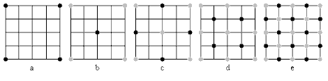
    Source: Reference [1]

Image A represents the initialization of 4 corner points of the landscape and is the starting point of the recursive algorithm. Each iteration is subdivided in 2 major steps:

Diamond Step – This step takes the square represented by the 4 corner points, computes the average using the value of these 4 points and adds a random value to it. This value is stored at the midpoint of the square, which is the intersection of the 2 diagonals. This results in diamonds when multiple squares are present in the grid. The diamond step is represented by Images B and D in the figure above.

Square Step – This step takes each diamond represented by the 4 points and calculates the midpoint of the diamond by averaging the values of the 4 points and adding a random value (of the same range as the diamond step) to it. The midpoints are the intersection of the diagonals of the diamond, which are essentially the midpoints of each of the edges in the original square (before the diamond step). The square step is represented by Images C and E in the above figure.

Each iteration is represented by 1 diamond and 1 square step. After every iteration, the amount of randomness added to the computed values is decreased so that we get a smoother terrain as we recursively go deeper into the landscape. This is done to get good critical points in the terrain that define the peaks and valleys in the landscape as well to get a good gradient when we go to higher iterations. The results section illustrates what we got from our implementation of this algorithm in hardware.

The pseudo algorithm for generating the fractal is as follows:
Initialize 4 corner points of the landscape.
While length of square side >= 1 {
     Pass through array that contains the squares and perform diamond step.
     Pass through array that contains the squares and perform square step.
     Add newly generated points to the array.
     Reduce the random number range
}

This gives a continuous terrain as it takes into account all values calculated by the neighboring squares and factors that in as well in midpoint calculations. The following is a software generated example terrain taken from Reference [1]:

 

Orthographic Projection

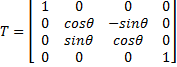
An orthographic projection was used to rotate the fractal landscape around the X axis using the following transformation matrix:

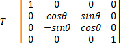
Since we were rotating in the negative direction, the signs were simply changed to

Hence the final computation using this matrix was:

Where

The point is represented in homogenous coordinates. Small x and y represent the pixel value of the landscape and z is represented by the height map/ intensity stored in the SRAM (as is explained by the following module). Hence, from this equation we observe that x pixel remains constant and only y is changing and z are changing for a particular angle. Since we want to keep the same intensity for the transformed landscape, we would not change the value of z. Thus, only y (or row value) will be changed in the algorithm and the equation that needs to be computed is as follows:

Thus, only 2 multiplications and 1 subtraction is required to compute the transformed value of each pixel. This concept was used in the orthographic module described in the section below.