High-Level Design
Source of Idea
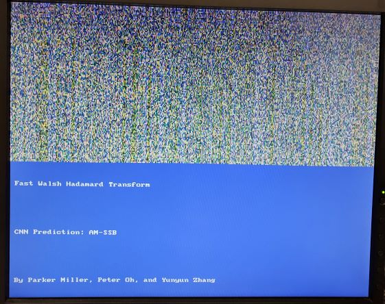
This idea for this project was inspired by the class competition of another course (ECE 4200) where the goal was to design a machine learning algorithm which could identify the modulation of various RF signals when provided their complex time domain values (also known as quadrature). Our group was also interested in neural networks so we decided to implement one of the more successful algorithms (a convolutional neural network) from that competition in hardware on an FPGA. As just feeding in test data from a dataset wasn’t a true application, we decided that this system should receive live radio data from a software defined radio. While this was relatively complex, we also wanted a means of visualizing the signals we received in order to provide a means of trying to tune the radio to find a signal with no prior knowledge. Originally we wanted to use an FFT spectrogram but realized that it would require too many multiplies to do in real time so we decided on the Fast Walsh-Hadamard Transform instead to get an alternative frequency domain representation that only relied on addition and subtraction.
Background Math
Quadrature (I/Q) Signals
In this report we refer to complex, quadrature, or IQ samples of a signal. This is a way that a signal can be decomposed into 2 values which can be used to find the amplitude and phase of a signal. I refers to the in-phase component and Q refers to the quadrature component (90 degrees out of phase). This convention allows the signal to be represented as the complex value I+jQ. As this is a complex number, now we know how to find the amplitude and phase of the signal. Though in this project we won't be using the amplitude and phase, but rather feeding I and Q data into the CNN and letting it determine ideal features for distinguishing the differently modulated signals. This is actually reasonable as when IQ data is plotted on the complex plane, it appears as an image which varies depending on the modulation used. Convolutional Neural Nets have been shown to perform well on image data, so we should expect reasonable results here too.
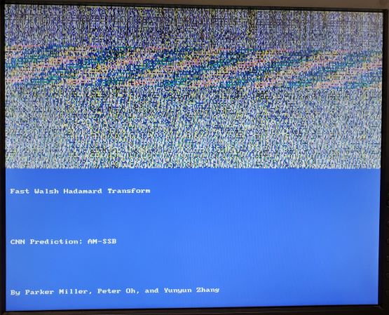
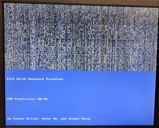
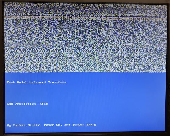
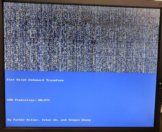
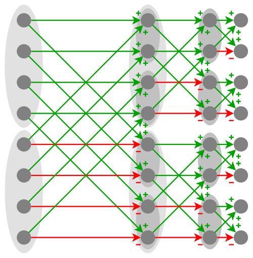
Fast Walsh-Hadamard Transform
The Walsh-Hadamard Transform is a generalized Fourier transform which decomposes a signal into a set of orthogonal signals. This is similar to a Fourier transform which uses sinusoids, though the Walsh-Hadamard Transform uses square/rectangular signals as it’s basis. Similar to how the fourier transform has an FFT for signals that are powers of 2 long, the Walsh-Hadamard Transform has the FWHT which does a similar decomposition to speed up computation on signals that are powers of 2 long. The actual transform is easily understood with the following image (from https://en.wikipedia.org/wiki/Fast_Walsh-Hadamard_transform):
A way to perform this recursive algorithm can be demonstrated with the following Python example code (from https://en.wikipedia.org/wiki/Fast_Walsh-Hadamard_transform):
            def fwht(a) -> None:
            """In-place Fast Walsh–Hadamard Transform of array a."""
            h = 1
            while h < len(a):
                for i in range(0, len(a), h * 2):
                    for j in range(i, i + h):
                        x = a[j]
                        y = a[j + h]
                        a[j] = x + y
                        a[j + h] = x - y
                h *= 2
Using this program and some formatted print statements, I was able to generate the verilog additions and subtractions required to apply the transform to a 128 sample long signal.
One thing excluded in this example code is a normalization factor of 1/sqrt(2) for each calculation. As this is applied to each calculation it can be factored out and even removed if desired as it scales the entire output equally (assuming you only care about the relative values of the transform outputs).
Weights Conversion
Once we had a model in TensorFlow that was simple and small enough for the FPGA, we stored all of the weights/parameters into a local .h5 file. Once this file was exported, we imported it into a jupyter notebook file and utilized python to format these weights into signed 18 bit (6.12 fixed point).
The .h5 file had 2334 total weights, all as floating point values.
We used a function float2fix(val, width, precision) that we found here: https://stackoverflow.com/questions/41590009/how-to-convert-a-float-point-number-to-a-fixed-point-number-with-a-certain-width

This function allowed us to format our floating point values into 6.12 fixed point.
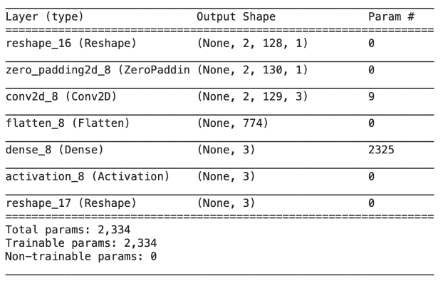
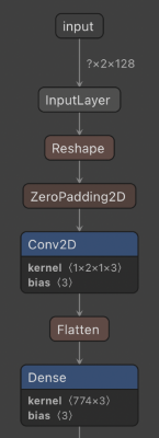
Convolutional Neural Network (CNN)
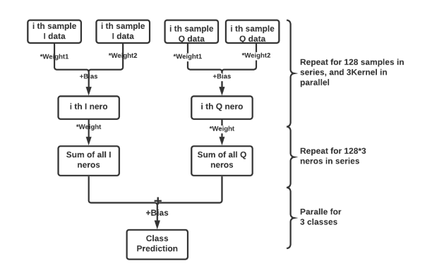
Convolution Layer Calculation: The convolution model we used in this project is the 2D convolution model. First, we added the [1,2] zero padding before and after the 128 samples to avoid information lost. The filter size in the convolution is [2,1], which means each neuron in the convolution layer will take two samples dot-product with the weight vector and add the bias term. For nth neuron in the convolution layer, [neuron_i, neuron_q]n = [w_i*nth sample_i, w_q*nth sample_q] + [bias_n, bias_n].
ReLu Function: ReLu stands for Rectified Linear Unit, the function is f(x) = max{0, x}.
Flatten Layer Structure: The flatten layer mainly flat the 3D matrix from the convolution output to 1D vector for the dense layer calculation. This layer first flats the kernel dimension, then with I, Q channels in this project, lastly flats with the signal samples.
Dense Layer Calculation:The input of the dense layer is a 1D flatten vector, and the output of the dense layer will be the 3 neurons, which represents the classification results for the 3 classes in this project. The mathematical representation of dense layer is Y = ReLu((weight input+bias)) for each class.
Logical Structure
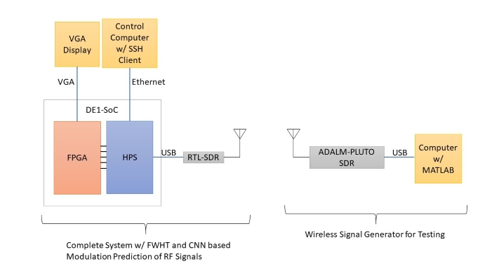
Our system has a few different parts which all need to communicate with each other to make sure processing completes fast enough such that a signal is received, processed, and displayed before the next 128 samples are ready.
This can be broken down into a few different components:
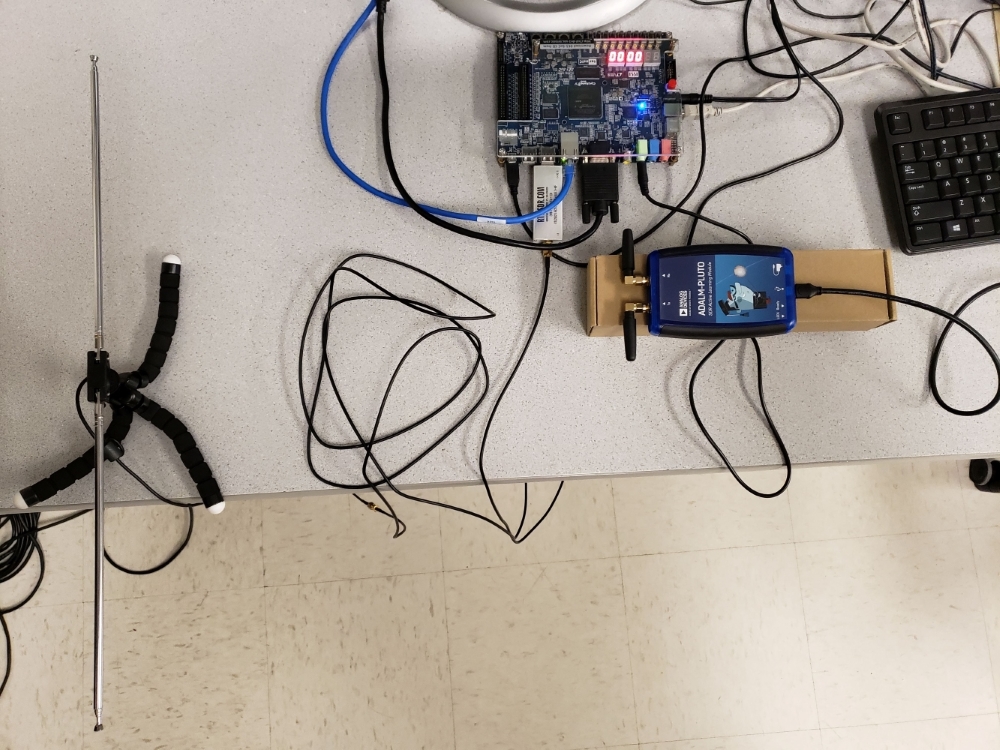
- RTL-SDR USB radio receiver
- HPS Linux System
- Our C program
- rtl_tcp program
- FPGA
- Main State Machine for Graphics and Data Reads
- FWHT Module
- CNN Module with Convolution and Dense Layers
The RTL-SDR is responsible for tuning to a specific RF radio frequency and sampling downconverted time domain IQ data.
The rtl_tcp program is responsible for controlling the RTL-SDR and sending those samples to a TCP client.
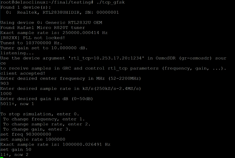
The C program we wrote on the HPS is responsible for retrieving the samples and writing them to the FPGA SRAM. It also is responsible for collecting user input for gain, sample rate and frequency settings for the SDR and sending them to rtl_tcp over TCP. Finally, it is responsible for resetting the FPGA as well as writing text to the VGA display.
The top level FPGA state machine is responsible for reading out the samples written to SRAM to a register bank and feeding them into the FWHT and CNN modules. Once the FWHT is complete, this state machine draws the output on the VGA display. After that, when the CNN is complete, it outputs the predictions to the HPS over a PIO port. Finally the state machine resets to start the process over for the next 128 samples.
Hardware/Software Trade-off
We utilized software to accomplish tasks that were not possible to accomplish on the FPGA as well as ones simplified design without slowing down real time processing. Tasks that were parallelizable or needed to be done in real time were delegated to the FPGA hardware.
Specifically the parts of our system written in software were the TCP client to retrieve data from the RTL-SDR and forward to the FPGA, the terminal user interface for changing SDR settings, and the VGA text code for displaying what the CNN is currently predicting.
The system elements written in hardware were the VGA display system (QSYS IP), VGA display of the FWHT, the FWHT itself, and the CNN. The FWHT and CNN had parallelized math operations while the VGA display had to operate quickly to maintain near real-time display updates.