We designed a gravitational N-particle simulator to solve Newton’s law of gravitation in full form and display a 3 dimensional representation of the particle’s interaction at high frame rates on a VGA monitor.
The purpose of our project is to simulate particles of different masses interactions with each other due to gravity. The system was designed to load any set of initial conditions. Additionally, the system displays a portion of 3-D space on a VGA monitor for visualization of the particle’s interactions. The third dimension is shown with color. The goal of the project was to simulate 1000 particles at a refresh rate of 10 Hz on one Altera DE2-115 board. All of the calculations are done in a 18 bit mantissa floating point format allowing any scale of initial conditions to be simulated.
High Level Design top
Rationale
Our main goal for our final project was to utilize all of the DE2-115’s logic elements and multipliers to perform otherwise costly computations at a reasonable power level and high speed. We decided to simulate gravity as Newton’s law of gravitation is straightforward but still requires many floating point operations. We wanted to make sure we were accomplishing something that would require the use of hardware processing elements and could not be achieved efficiently with a simple processor.
Logical Structure
Our design is essentially focused around a Nios II processor. This project is bottlenecked by memory access speeds on the DE2-115 boards as we need to fetch particle’s information repeatedly. A Nios processor was chosen as the memory controller for simplicity while not sacrificing much speed. The gravitational calculations are performed in a floating point format to allow a wide range of particle distances and masses to be simulated. As a result, the Nios processor would be bottlenecked attempting to do all of the floating point math. We made a hardware computational module which is loaded with the particle’s parameters and has all the necessary floating point hardware to compute the multiplications, inverse square root, and additions required to complete the computations. We are also able to cut down on repeated memory accesses by running many computational modules in parallel, which receive the same particle information reducing memory accesses almost by a factor of the number of modules. The parallelization and speed of the processors is what enables us to compute large amounts of particles quickly with just a Nios processor controlling memory. Additionally, the Nios also updates the VGA display with the particle’s positions in a 3-dimensional representation. The last function the Nios performs is to load the particle’s initial conditions through Matlab through RS232.
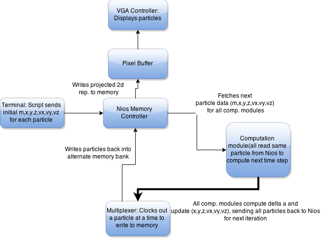
Block Diagram
Hardware/Software Tradeoffs
Hardware was used only for the computational engines as we were able to instantiate lightweight floating point modules to compute the multiplications, additions, and inverse square root steps. These would be incredibly slow to do on in software. Alternatively we could have given the Nios a FPU but this would not have been parallelizable (which is what gives the project lots of speed as it greatly reduces repeated memory accesses). A Nios soft core was used to drip and load particles to the engines, acting as the memory controller. This was a simple and still fast way to streamline memory accesses. The Nios also reads initial conditions over RS232. Software was used as scanf() is already written for C, making implementation easy. Our VGA screen was also updated by the Nios because of the simplicity of adding the VGA controller to SOPC builder.
Background Math
Our simulator revolves around Newton’s law of gravitation which is shown below:
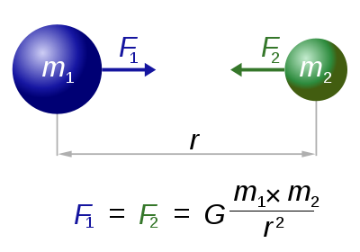
Newton's law of universal gravitation
It states that there is an attractive force between any two objects with masses proportional to the mass and the inverse square of the distances between them. For our project we assume all particles are point masses and as such can not collide. We use Euler integration in order to generate our discrete frames. The simulation is run much faster than the particles are moving relative to their distances, resulting in an accurate approximation of the trajectories of the particles at any time step. The resultant force vector is calculated from the interaction of every particle with every other particle and no approximations are made here resulting in O(N^2) computations.
More specifically, we calculate the acceleration for a particle shown below. This equation calculates the acceleration for a single particle based on the position and mass of all the others. This acceleration is then used to calculate the updated velocity and position.
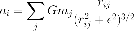
Acceleration Equation
Intellectual Property
The Nios II and all of its peripherals are Altera IP cores, and some of the peripherals are part of the University Programs IP cores.
Our design is loosely based on the Gravity Pipe (GRAPE) project out of TOkyo Univeristy. The project is a does gravitation calculations with many simple processors utilizing SIMD (Single Instruction Multiple Data). The papers writting about the project helped us begin to think of an efficint way to completing our task on the FPGA.
We also implemented our floating point from a modified version of one implemented by Skyler Schneider here. Ours is modified to more closely resemble the IEEE standard.
Hardware top
Hardware Overview
The hardware for the project is very straight forward. It consists of a nios softcore processor, gravity computation engines, and some muxing logic to let the processor select an output to read. The gravity engines are built around custom 27-bit floating point hardware and a simple state machine. The engines receive inputs from the controller and send their outputs to a mux that the controller controls.
Floating Point
The floating point hardware is a stripped down version of the IEEE single precision floating point standard. It is 27-bits and formatted as follows:
- bit 26: Sign
- bits[25:18]: Exponent
- bits[17:0]: Fraction
An exponent value of zero is how zero is represent in this format. There are no infinity, denorm, or NaN representation in this floating point representation. The value of any other is calculated as shown.

Floating point value
The floating point operation included are addition/subtraction, multiplication, and inverse square root. Addition is a 2-stage pipelined module, multiplication is a combinational module, and the inverse square root is a 5-stage pipelined module. The inverse square root module uses the fast inverse square root algorithm documented here. This provides a much faster alternative than the traditional floating point algorithm. With one iteration of Newton's method, the result is within a few tenths of a percent of the actual value. A second iteration can be done to make the result even more accurate if needed.
Gravity Engine
The engine that does that gravity calculations follows the state machine shown below. It was implemented this way because a transition to a fully pipelined design would follow the same flow but there would be registers between states and duplicated floating point arithmetic hardware. The pseudo-code for the engine's calculation is shown.
for (i = 0; i
< N; i++) {
for (j = 0; j
< N; j++) {
if (j != i) {
rx = p[j].x - p[i].x;
ry = p[j].y - p[i].y;
rz = p[j].z - p[i].z;
dd = rx*rx + ry*ry + rz*rz + EPS;
d = 1 / sqrtf(dd * dd * dd);
s = p[j].m * d;
a[i].x += rx * s;
a[i].y += ry * s;
a[i].z += rz * s;
}
}
}
The inputs to the controller are mostly as expected. It receives the position, velocity, and mass of the particle to be loaded or used for calculation. Load, Go, and Reset are control signals to let the engine know when to store the values, begin a calculation, or reset. The engine number is also an input so it can compare it and determine if the controller is trying to communicate with it or some other engine. The final input is the stop number. This number is used to determine when the calculation is complete and the engine can compute the new velocity and position to output. The engines output the new velocity and position, and it also has 2 status signal to let the controller know when it is done with the whole calculation, or ready for a new particle. The engine state machine is shown below:

Engine FSM
IDLE: In the idle state the engine is waiting for the controller to load a particle or send the go signal to start the calculation.
CALC 1-2: States calc1 and calc2 do the calculations for rX, rY, and rZ.
CALC 3: State calc3 calculates rX^2, rY^2, and rZ^2.
CALC 4-7: States calc4 to calc7 complete rX^2 + rY^2 + rZ^2 + EPS.
CALC 8-9: States calc8 and calc9 complete dd*dd*dd.
CALC 10-14: These 5 states are needed for the inverse square root calculation.
CALC 15: This state calculates s = p[j].m * d.
CALC 16: Calc16 computes s*rX, s*rY, and s*rZ.
CALC 17-18: These 2 states add the previous results to the corresponding acceleration value.
CALC 19: The final calculation state store the accelerations and determines if the engine has gone through all of the particles. If it is done it continues to the done1 state and starts to calculate the updated velocities. If it isn’t done, the state goes back to idle and waits for the controller to input a new particle.
DONE 1: This state just waits for the velocities to finish in the adders.
DONE 2-3: Using the new velocities, these 2 states calculate the new coordinates.
DONE 4: The final state sets the outputs and lets the controller know that it is done with the computation.
Software top
Nios II Memory Controller
The C program which controls the computational engines is very simple and follows a state machine flow. All variables and peripherals are set up initially and then the program goes to the reset state. The state machine is shown below:
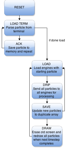
Nios FSM
RESET: The program is rest to the point where it is ready to receive a new set of particle initial conditions from the terminal.
LOAD_TERM: Here the program waits for the terminal to output a string with a terminating character. If the first character is a ‘p’ the data following is the particle initial condition and this is saved into memory. If the first character is a ‘d’ this means the terminal is done sending particles and the state machine can proceed to computation. The Nios ACKs every string sent by the computer except for the “done” string.
LOAD: This is the first state in setting up the computational engine. The way the engines work is they are first given a particle which they will be computing the net force due to all other particles interaction. The LOAD state is where each computation engine is addressed and given its particle. This is iterated once for every engine.
DRIP: Once each engine receives the particle they will be computing for it must sequentially compute the individual acceleration components due to each particle on it. In the dripping state we send every particle to every engine in parallel. This method decreases the number of particle memory accesses by a factor of the number of engines. The controller waits for all the engines to be ready for the next particle before it fetches the next particle.
SAVE: Once all the particles have been dripped to the engines the computational engine has calculated the resultant acceleration on the particle that was initially loaded to it. All engines output the new particle state (x,y,z,vx,vy,vz) back to the controller and the controller sequentially toggles a hardware multiplexer while reading it parallel ports and saving the newly computed values back into our second particle state buffer. If the next state for all N particles have been computed then the VGA controller will update the screen and the program proceeds to the DRAW state. If we still have more particles to load and save then we go back to the load state and continue where we left off.
DRAW: Once all particles have been saved we update the VGA screen. The program waits for the vertical sync pulse as this is a safe time to update the VGA buffer with not flicker. If the LOAD/DRIP/SAVE states execute fast enough the VGA screen will update at 60 FPS. If they are not fast enough the VGA buffer will be updated at the next vertical sync pulse. First we take our floating point x,y,z positions and do a fast cast to integer. Next the program waits for the vertical sync pulse. Then the program erases the old particle position and draws the new particle. Boundaries are checked and only particles within a 640x480x640 box are drawn. The z dimension is represented by a color shade. Particles located at z=320 are white and they fade to red/green respectively as they move further or closer from the z=320 plane. The last step in drawing is calculating the VGA frame rate as this is one of our project’s metrics. The total number of frame updates in one second is displayed in the bottom left of the screen.
Reference design/code
We referenced a common site template used by many groups have used in the past. This template originates back to the Human Tetris project from 2010.
Results top
Failed Attempts
This project actually came together very smoothly as we spent lots of time planning out the structure of the design and were about to make it work without significant design changes. We had a hard time getting the RS232 connection to work to load initial conditions. We started with JTAG UART interface but as it turns out this is not accessible by Matlab or any other terminal program. As a result we had to switch to using the RS232 interface. This worked simply but we had problems reading characters for it. Originally, we tried to implement our own character scanner to read in strings. For some reason it did not operate fast enough and we had to add a large pause (10ms) between characters for it to work. This was not acceptable as we had to transmit a large amount of data. We spent lots of time getting the board support package to make the built in C scanf function work with RS232. It turned out that JTAG UART is the default scanf device and if you remove it and leave RS232 it will become the default. We were able to receive data at 115kbits in the end though.
We also tried to increase our clock rate to 100MHz for the Nios, SDRAM, and engines but the project did not work and we were not able to spend enough time to figure out where we made a mistake.
Speed of Execution
When we are simulating 1000 particles we are able to achieve 147 MFLOPS. The VGA monitor is able to update at 60 frames per second at low particle counts. However, with 1000 particles drawn as points we can achieve an update rate of 7-8 FPS. This is very close to our goal of 10 FPS and could easily be achieved with a clock rate increase as we are running everything at 50 MHz. There is no flicker on the VGA monitor and the particles appear to move very smoothly given suitable initial conditions.
Accuracy
The first and most important note to make about accuracy is the use of the fast inverse square root algorithm. This algorithm does a very good job at making an initial approximation and then does one iteration of Newton's method to make the result even better. With one iteration, the result is within a few tenths of a percent to the actual value. T make the result even more accurate, another iteration can be done, however, from our experience, one iteration was enough to produce expected orbits and gravitational effects.
The next concern for accuracy is the use of an 18 bit mantissa for floating point instead of the normal 23-bit used in the IEEE single precision standard. This provided us with more precision than we needed and also gives a huge dynamic range for possible positions, velocities, and masses. Most scenerios could be input as initial conditions in our simulator.
Usability
Our design is very usable by other people as once the FPGA and Nios are programmed one only needs to run a Matlab program which outputs particles in the correct format and transmit the start frame. The matlab program can be modified by anyone easily with different initial conditions (x,y,z,vx,vy,vz,m)
Conclusions top
We were able to come extremely close to meeting our expectations for the project. Our goal was 1000 particles at 10 FPS and we were able to achieve 1000 particles at 8 FPS. However, we only scratched the surface of what we could do with that FPGA. We utilized almost all of the FPGA but there would have been more efficient ways to do the computations.
Potential Changes
The first thing we would change is clocking the Nios and computational engine modules much faster than 50 Mhz. We could easily double our throughput with this change. We attempted to speed everything up but it did not work and we did not pursue it any further as it is a trivial way to get more speed and not the goal of our project as we were running out of time
The second major change we could have is to speed up memory accesses. We did not put much thought into this other than reasoning that the Nios could handle the memory accesses in a reasonable amount of time to get 1000 particles on the screen. A hardware module could be used to speed up the memory accesses. However, the way it is currently written the Nios controller is fetching the next particle while the engine is computing the previous one, resulting in an efficient implementation. A faster memory would be useful for this project.
The last change we would make is to change the computational engine from a state machine to a pipeline. We considered doing this to increase our throughput but when you consider how slow the Nios’s memory is we would not be able to load enough particles into the engines to fill the pipeline at a faster rate. As such, parallelizing the engines greatly reduces the effect of the slow memory access speeds by eliminating a large amount of accesses. Additionally, a pipelined engine would not be able to use the same floating point modules in every stage and would have a much larger footprint, reducing how many engines we could have. If we had a lower latency way to access memory a pipelined engine would make a larger difference.
Appendices top
A. Source Code
Python Script - to run: python gravityEngine.py [# engines] [output file]
B. Division of Labor
| Task | Completed By |
|---|---|
| Floating Point Hardware Verilog | Mark |
| Computational Engine Verilog | Mark |
| Nios Controller C | Brian |
| Matlab initial conditions script | Brian |
| Engine instantiation python script | Mark |
| General Debugging | Mark/Brian |
Created with the HTML Table Generator
References top
This section provides links to external reference documents, code, and websites used throughout the project.
Datasheets
References
Background Info
Acknowledgements top
We would like to thank Professor Bruce Land for teaching an amazing course, and anyone in lab who helped with random problems throughout the course