Two-Player Boids Game
With Laser Pointer Controllers
Claire Caplan (crc235), Alec Wyatt (acw254) & Shreyas Renganathan (sr2322)
Demonstration Video
Objective
Our project extends the boids algorithm into a two-player game in which players compete to “eat” the most boids by each steering a predator using a laser pointer tracked by computer vision.
Introduction
We have created a game based on the principles of the boids algorithm introduced in Lab 2. The game involves two players standing in front of a projector screen full of boids, each player taking on the role of a predator and using a laser pointer to control the predator’s position. The object of the game is for each player to “eat” as many boids as possible by steering their predator around the screen with a handheld laser pointer. When a boid is eaten, players see a “splat” on the screen when the boid disappears and hear a beep corresponding to their laser pointer color. Players can see the current position of their predator on the screen. Once all boids are gone, the player that has eaten the most boids wins the game. For safety in the presence of lasers, all spectators must stand behind the players (see the Safety section below).
The game uses the PIC32 as the main host of the game, a Raspberry Pi to run computer vision and track the laser pointers, a pair of laser pointers held by the players to control the positions of the predators, a webcam to track the positions of the laser pointers on the screen, a document camera to capture the thin film transistor (TFT) display, and a projector to display the game on a large screen.
A Raspberry Pi with a webcam uses computer vision to track the laser pointers. One player carries a red laser pointer, and the other uses green. The two laser pointers are differentiated by their color contents in the computer vision program. The Raspberry Pi uses the open-source opencv library in python to locate the laser pointers and produce an (x, y) coordinate pair representing the position of each laser pointer mapped to a position on the TFT. The Pi sends this pair of coordinates to the PIC32 over a serial interface.
The PIC runs the boids algorithm, executes the game procedure, and positions the predators in relation to the laser pointer coordinates sent by the Pi. The PIC runs an optimized boids algorithm for the prey boids, but it runs an augmented set of logic to control the positions of the predators. The PIC takes in the coordinates provided by the Pi in the calculation of new predator positions. The coordinates sent by the Pi represent points that the predators turn toward with a limited acceleration and velocity. The farther the pointer coordinate is from the predator’s current position, the faster the predator’s speed will become. This coordinate-to-predator relationship will be employed instead of using the coordinate as a simple position vector for the predator both to make the motion of the predator more organic and boid-like and to make the game more fair by subjecting the predators to some constraints on their velocity.
The project required significant augmentation of the boids algorithm and completely new logic for controlling the predators and executing the game. It also required implementing fast and reliable communication from the Pi to the PIC. This proved to be the most technically challenging and time-consuming part of the project. The result is an exciting and entertaining game which stresses multiple aspects of the PIC32’s capabilities.
High Level Design
After completing Lab 2, we believed the boids algorithm we developed could be extended into an interactive, entertaining game that would stretch the capabilities of the PIC 32, integrate new hardware and software complexity using a Raspberry Pi and computer vision, and augment our experience in using techniques such as direct digital synthesis (DDS), threading, code optimization, and serial communication. The final product works almost exactly as outlined in the Final Project Proposal, with two players competing to eat 40 boids rendered on the big screen in Phillips 101. The project was inspired by the idea that a game could be designed in which all of the intelligence is removed from the game controller, leaving behind an intuitive interface in which the player must simply point to where they want their predator to travel. We envisioned a game which would complement the natural human tendency to point where we want an object to go rather than abstracting the user input into a joystick or contrived controller. Such a game also enables a player to play from almost any distance or position as long as they have a line of sight to the screen. This type of design requires more intelligence at the point of gameplay and more complexity. The Raspberry Pi is needed to identify the positions of the pointers and communicate these coordinates to the PIC, and the PIC must operate on these inputs to place the predators according to the user’s inputs. The result is an intuitive, fluid user interface.
The high level system block diagram is shown in Figure 1.
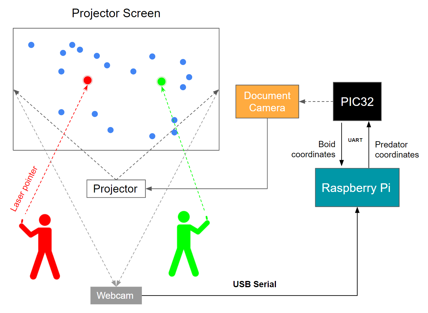
Figure 1. High Level System Block Diagram
Boids Algorithm Background Math
The following pseudocode describes the operation of the game. It is adapted from the ECE 4760 course website.
# For every boid . . .
for each boid (boid):

# Zero all accumulator variables
xpos_avg, ypos_avg, xvel_avg, yvel_avg, neighboring_boids, close_dx, close_dy = 0

# For every other boid in the flock . . .
for each other boid (otherboid):

    # Compute differences in x and y coordinates
    dx = boid.x - otherboid.x
    dy = boid.y - otherboid.y

    # Are both those differences less than the visual range?
    if (abs(dx)<visual_range and abs(dy)<visual_range):

        # If so, calculate the squared distance
        squared_distance = dx*dx + dy*dy

        # Is squared distance less than the protected range?
        if (squared_distance < protected_range_squared):

            # If so, calculate difference in x/y-coordinates to nearfield boid
            close_dx += boid.x - otherboid.x
            close_dy += boid.y - otherboid.y

        # If not in protected range, is the boid in the visual range?
        else if (squared_distance < visual_range_squared):

            # Add other boid's x/y-coord and x/y vel to accumulator variables
            xpos_avg += otherboid.x
            ypos_avg += otherboid.y
            xvel_avg += otherboid.vx
            yvel_avg += otherboid.vy

            # Increment number of boids within visual range
            neighboring_boids += 1

# For every predator . . .
for each predator (predator):

    # Compute the differences in x and y coordinates
    dx = boid.x - predator.x
    dy = boid.y - predator.y

# Are both those differences less than the death range?
    if (abs(dx)<death_range and abs(dy)<death_range):

squaredpredatordistance = dx*dx + dy*dy

if (squaredpredatordistance < deathrange*deathrange):
       # If so, this boid gets eaten
          boid.eaten = 1

  if (predator.id == 0):
    score1 += 1
  else:
    score2 += 1


    # Are both those differences less than the predatory range?
    if (abs(dx)<predatory_range and abs(dy)<predatory_range):

        # If so, calculate the squared distance to the predator
        squared_predator_distance = dx*dx + dy*dy

        # Is the squared distance less than the predatory range squared?
        if (squared_predator_distance < predatory_range_squared):

            # If so, accumulate the differences in x/y coordinates to the predator
            predator_dx += boid.x - predator.x
            predator_dy += boid.y - predator.y

            # Increment the number of predators in the boid's predatory range
            num_predators += 1

# If there were any predators in the predatory range, turn away!
if (num_predators > 0):
    if predator_dy > 0:
        boid.vy = boid.vy + predator_turnfactor
    if predator_dy < 0:
        boid.vy = boid.vy - predator_turnfactor
    if predator_dx > 0:
        boid.vx = boid.vx + predator_turnfactor
    if predator_dx < 0:
        boid.vx = boid.vx - predator_turnfactor

# If there were any boids in the visual range . . .
if (neighboring_boids > 0):

    # Divide accumulator variables by number of boids in visual range
    xpos_avg = xpos_avg/neighboring_boids
    ypos_avg = ypos_avg/neighboring_boids
    xvel_avg = xvel_avg/neighboring_boids
    yvel_avg = yvel_avg/neighboring_boids

    # Add the centering/matching contributions to velocity
    boid.vx = (boid.vx +
               (xpos_avg - boid.x)*centering_factor +
               (xvel_avg - boid.vx)*matching_factor)

    boid.vy = (boid.vy +
               (ypos_avg - boid.y)*centering_factor +
               (yvel_avg - boid.vy)*matching_factor)

# Add the avoidance contribution to velocity
boid.vx = boid.vx + (close_dx*avoidfactor)
boid.vy = boid.vy + (close_dy*avoidfactor)


# If the boid is near an edge, make it turn by turnfactor
if outside top margin:
    boid.vy = boid.vy + turnfactor
if outside right margin:
    boid.vx = boid.vx - turnfactor
if outside left margin:
    boid.vx = boid.vx + turnfactor
if outside bottom margin:
    boid.vy = boid.vy - turnfactor

# Calculate the boid's speed
# Slow step! Lookup the "alpha max plus beta min" algorithm
speed = sqrt(boid.vx*boid.vx + boid.vy*boid.vy)

# Enforce min and max speeds
if speed < minspeed:
    boid.vx = (boid.vx/speed)*minspeed
    boid.vy = (boid.vy/speed)*maxspeed
if speed > maxspeed:
    boid.vx = (boid.vx/speed)*maxspeed
    boid.vy = (boid.vy/speed)*maxspeed

# Update boid's position
boid.x = boid.x + boid.vx
boid.y = boid.y + boid.vy

# For every predator . . .
for each predator (pred):

# Compute distance to laser pointer
dx = laser.x - predator.x
dy = laser.y - predator.y

# Update predator position
predator.x =  predator.x + (dx*pred_speed_factor)
predator.y - predator.y + (dy*pred_speed_factor)
Predator Lag Background Math
The boids algorithm is an artificial life algorithm, meaning it models the emergent behavior of groups of living creatures subject to physical constraints on their movements. If the predators in our boids game tracked the positions of the laser pointers exactly, then with a flick of the wrist a game player would be able to move their predator across the entirety of the screen, producing an unrealistic predator motion and making the game far too easy. To remedy this problem and cause the predators’ motion to more closely match that of the boids they are pursuing, we created a “laggy predator.” Instead of the laser pointer encoding a position vector for the predator, it is instead used to describe a position to which the predator flies. The farther from the laser pointer the predator is, the faster it flies toward the pointer. As it approaches the pointer position, the predator gradually moves slower. In a given frame, the predator can move at most the distance to the laser pointer multiplied by a factor called the predspeedfactor. In this way, the difficulty of the game can be tuned by adjusting the predspeedfactor.
Computer Vision Background Math
We designed a computer vision system on a Raspberry Pi to parse player input and send it to the PIC32. The system receives a stream of image frames from a webcam, applies image processing to isolate two laser pointer dots in each frame, and estimates their positions within a region of interest mapped to the TFT display. It then transmits those positions to the PIC32 continuously via UART.
We chose to implement OpenCV tools in Python to develop this. While OpenCV is also available in a C++ implementation, its Python implementation abstracts away several steps that have to be manually performed in the C++ implementation. While minimizing the risk of misconfiguration in this manner, the Python implementation has also been highly optimized as a wrapper around C++ functions. Therefore at moderate frame rates (around 20fps), performance is nearly identical between both implementations. The worst-case difference in execution time between the two is only around 4% [3].
For rapid transfer of predator coordinates to the PIC32, we wanted to achieve reliable object detection and localization with minimal latency. So our design approach was to use OpenCV’s native functions as much as possible, while minimizing the number of pixels (using spatial and colorimetric filtering) to be processed by those functions.
The pseudocode design for the computer vision algorithm is shown below.
while (program is active):

        # Grab new video frame (image) from webcam
        # Mask out (i.e. set to zero) pixels outside of the rectangular region of interest
        #Set lower and upper bounds in color space for each laser pointer color

        for each laser in colors:
                # Create a copy of the image
                # Mask out pixels whose values are outside the respective color space passband
                # Process the image as necessary using OpenCV tools to isolate the dot
                # Virtually draw the smallest circle that encloses the dot
                # Estimate the centroid of that circle
                # Map the centroid coordinates to the PIC32’s mapping of the TFT screen
                # send laser color’s coordinates to the PIC over UART
                serial.send(laser_color_id, x, y)
Logical Structure
The logical structure of our final product involved separating processing tasks as much as possible between the PIC32 and the Raspberry Pi, with minimal communication between the two devices. The Raspberry Pi was solely responsible for computer vision tasks to determine the positions of both players’ laser pointers, and this was achieved through connecting a webcam to the Pi which ran Python code using the OpenCV library. The PIC32 was responsible for performing all of the mathematical calculations relevant to the boids algorithm, as well as rendering all TFT animation elements and playing sounds through direct digital synthesis. The connection between these two devices was designed to be as simple and fast as possible, with serial communication occurring over UART to send each laser pointer’s ID, x, and y coordinates from the Pi to the PIC.
Hardware/Software Tradeoffs
Since our project heavily focused on animation and computer graphics algorithms, our goal was to make the hardware aspects of the project as simple as possible. This drove our choice to split the software tasks between two different computing components, the PIC32 and the RaspberryPi. We knew that the Pi would be critical in implementing OpenCV. Since we also wanted a hardware-minimal way to connect to a projector, we also opted to try rendering our game elements on the Pi as well by sending them from the PIC. As a result, our only connection through hardware between the two microprocessors was over UART serial communication, which we hoped would simplify the hardware as much as possible. Our only other hardware connection was over USB, to connect an off the shelf webcam to the Pi for computer vision.
Relationship to Standards
Since we are not transmitting anything wirelessly in our implementation, we do not need to account for or apply any IEEE or likewise standards.
Program/Hardware Design
Our project involved both C code running on the PIC32 microcontroller and Python code running on a Raspberry Pi, which will be discussed in depth in the following sections.
PIC32 Program Design
For the final version of our game, we ended up implementing both the mathematical calculations for the boids algorithm and the game display elements in C to run on the PIC32. Since we were basing our game around the boids algorithm, we started with the lab 2 code as a framework. This also included support for one predator, since we implemented the MEng version of the lab. The boids algorithm achieves realistic flocking behavior by adjusting the velocity of each boid according to the following parameters common to all boids: turn factor, visual range, protected range, centering factor, avoid factor, matching factor, maximum speed speed, and minimum speed. The turn factor dictates the turn radius the boids can achieve, with a greater turn factor leading to a tighter turn radius and flocking behavior that appears more “bouncy.” The visual range is the distance at which a boid can detect and act upon the presence of other boids; a greater visual range allows the boids to coordinate their velocities more tightly with the boids around them, and thus flocks become more homogeneous in their movement. The protected range is a measure of the personal space asserted by each boid, with a larger protected range leading to wider spacing in the flock. The centering factor is the boids’ affinity for gravitating toward the other boids within the visual range, with a greater centering factor drawing the boids more tightly together. The avoid factor encodes the strength of the avoidance behavior. The maximum and minimum speeds place bounds on boid velocities to mimic more realistic behavior.
In our lab 2 code, we managed boids and our single predator through the following struct:
typedef struct
              {
                _Accum x;
                _Accum y;
                _Accum vx;
                _Accum vy;
                } boid_t
Since our game involves determining whether a boid has been eaten so that it can be removed from the screen and added to a player’s score, we modified this struct to include an ‘eaten’ flag for each boid_t object:
typedef struct
              {
                _Accum x;
                _Accum y;
                _Accum vx;
                _Accum vy;
                int eaten;
                } boid_t
As in lab 2, we had an animation thread to handle animation calculations and TFT rendering. In the beginning section of the thread, we initialized a boid array of size 40, with boid positions and velocities initialized randomly using the same rand() functions as in lab 2. Additionally, to support two predators for our two player game, we initialized a predator array in a similar manner. Both boid and predator objects use the same boid_t struct since they all move using x and y positions and velocities. While predators do not use the eaten flag, the flag is initialized to zero in all boid_t objects and will just never be modified for boid_t objects belonging to the predator array. Finally, the beginning section includes drawing 4 lines onto the TFT at the screen edges in order to clearly visualize the game field edges for the players.
The looping section of the thread was also structured very similarly to the lab 2 code, following the pseudocode algorithm described in the previous section. In order to determine positions for all of the boids, we have a nested for loop with multiple subsections. The highest level loop iterates over all of the boids in our boid array. If this boid has not been eaten, we proceed into the other layers of the loop to determine its next position according to the boids algorithm. We erase the boid by drawing a black pixel in its original position. We then determine a new position relative to all of the neighboring un-eaten boids in the boid array, as described in the pseudocode in the last section. We then iterate over both predators, and determine the boid’s final new position following the algorithm’s rules for how boids should avoid predators.
Then, in the next loop we iterate through the predators once again to determine how close the boid is to both predators. If a predator is within the proximity of the predefined variable deathrange, we set the boid’s eaten flag to 1 so that it will not be rendered again. We then add the boid to the score variable of that predator. If the sum of both players’ scores is equal to the number of boids in the game, we display a winner’s screen for the winning player, along with the final score and pass into an infinite while loop so that the game will effectively end until it is reset. This is shown in Figure 2. At the end of the loop, we proceed to render all of the gameplay elements each time, including the scores of both players in the top corners of the screen, and the boundary lines, since they may have been erased by boids that “flew” over them. If a boid has been eaten, we also animate it such that it appears to explode over a sequence of 4 cycles. Each time the eaten boid is rendered, its radius will grow and the eaten flag will be incremented to reflect its status in the explosion animation cycle. Once the eaten flag reaches a value of 4, the boid will be rendered in black for the rest of the game. Finally, to increase the difficulty of the gameplay as the game goes on, we check the combined score of the players to determine how many boids are left, and progressively increase the value of the predatorrange variable so that boids are able to “fly away” from the predators at further ranges. At the very end of the looping section, we save the updated boid with its new positions and eaten flag value back into the same spot of the boid array.
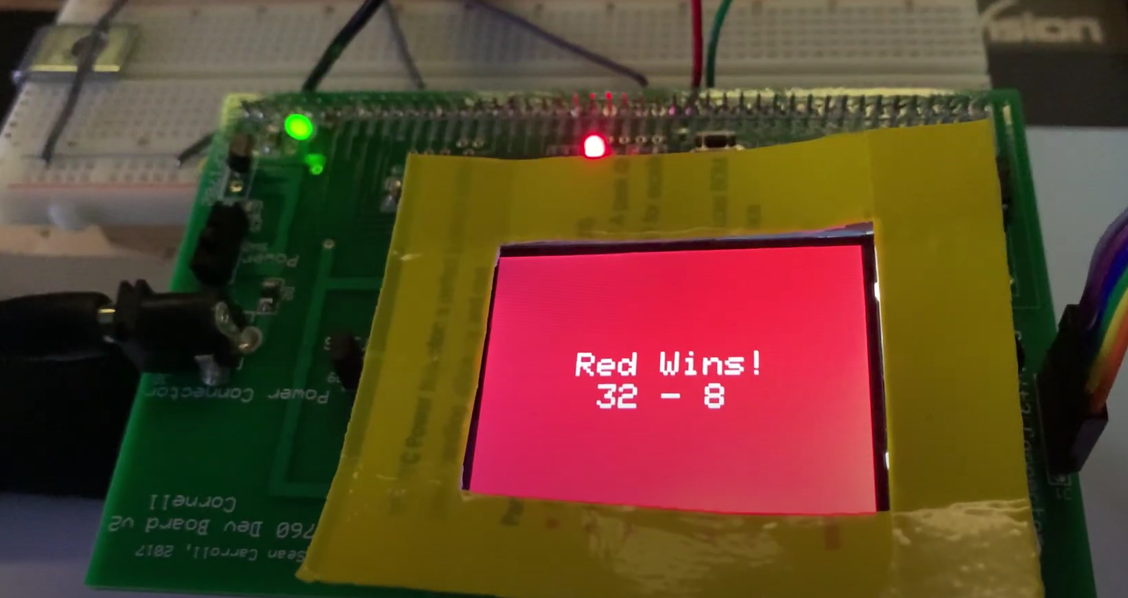
Figure 2. Game end screen showing winner and final score
In addition to our animation thread, we also carried over the structure of the Python string reading thread and serial thread from lab 2. Instead of taking serial inputs from a GUI, we performed the same serial sending method within our OpenCV python script to pass the coordinates of the players’ laser pointers. We maintained the same serial thread as the lab 2 example code to set a flag whenever a new string was in the receive buffer, and removed all other extraneous elements of the thread since we did not need to handle buttons, sliders, or any other GUI elements. In the Python string thread’s loop section, we began by reading in the received string from the buffer and separating it into a predator ID (ID 0 for the green laser and ID 1 for the red laser), along with the laser’s x and y position. We then pulled the correct predator object from the predator array using the ID, and drew black over its current position. Using the lagging predator math described in the previous section, we then calculated updated x and y coordinates of the predator based on the laser pointer coordinates and the predator’s current velocity. Then the new predator was drawn as a circle or a square (for player 1 and player 2, respectively) at the updated coordinate location, and the updated predator object was saved back into the array.
Finally, to enhance our gameplay experience further, we added different sound effects for each predator which played each time that predator ate a boid. We achieved this via direct digital synthesis as in lab 1. Using the same ISR structure as in lab 1, we were able to trigger a sound synthesis interrupt each time a score was incremented in the animation thread by setting note time to 0. In addition, depending on which predator consumed the boid, we set the sound variable to either 1 or 2. This resulted in playing either a 330 Hz or 440 Hz short tone for player 1 or player 2, respectively.
Our original goal was to achieve 2 way serial communication between the PIC32 and the Raspberry Pi, and have the Pi render the game elements so that we could connect to a projector via HDMI. Ultimately, we ran into a variety of issues in achieving two-way communication at a high enough speed to render the whole game in a visually appealing manner, and in our final demonstration we rendered the game onto the TFT screen and projected it in Phillips 101 via a document camera, which worked very well as a quick solution.
While quantitative aspects of our efforts to achieve communication are described further in the results section, we did code our gameplay rendering in a variety of different languages and libraries in each of our different attempts. Our original method was to send each boid’s coordinates and boid ID number from the PIC to the Pi over serial, and read them on the Pi side using the readline() function from the Pyserial library. The rendering of each game element would then occur in Pygame, which we knew to be extremely lightweight since it was written as Python calls down to basic C functions, and we had significant experience and success with the library in projects for ECE 5725. However, we noticed that even with a few boids in the game we would get significant delay and very low frame rate, and after some online research we attributed this delay to the readline() function. We then experimented with a faster implementation of the readline function which was built around the Pyserial read() function, but saw very little improvement. Finally, in a last ditch attempt to make Python work for our rendering and communication scheme, we implemented a serial read program in C using the WiringPi library, which we ran on the Pi to read serial transmissions into a named pipe in Linux. From the named pipe, we attempted to read in and pass information to Pygame, however we still experienced significant lag and poor animation performance. After exhausting our Python implementation options, we then turned to C++ in hopes of achieving faster rendering and reading speeds that could keep up with the PIC’s communication speed and achieve a 30fps frame rate. After extensive research and experimentation with different example animation programs on GitHub, we chose to use the Simple Fast Multimedia Library (SFML). We found a bouncing ball animation in SFML on GitHub, and extended the object oriented nature of this code to make the ball class render both boids and predators. We also tied in the WiringPi library to perform serial reads directly into the game program, without a named pipe as a conduit. Ultimately, this performed significantly better than our Python implementations, and we were able to achieve a visually passable frame rate with just a few boids. However, when we added boids to the game our frame rate decreased exponentially, and had extremely large lag in animation after about 10 boids. At this point, we elected to pivot to using the document camera in our final demonstration, since we had about a week left to work on the project and had yet to implement any gameplay features or integrate with the OpenCV laser tracking system.
Raspberry Pi Program Design
The computer vision algorithm was successfully developed as a set of Python scripts, based on OpenCV, running on a Raspberry Pi 3.
First, after several unsuccessful attempts to compile an OpenCV version with a dependency set compatible with a Raspbian Buster image on a Raspberry Pi 3, we eventually found a third-party-maintained, pre-compiled version of OpenCV 3.4.6.27 that installed correctly for Python 3.
The successful install was performed as follows:
sudo pip3 install opencv-contrib-python==3.4.6.27 -i https://www.piwheels.org/simple
              sudo apt-get update -t buster
              sudo apt-get install libhdf5-dev -t buster
              sudo apt-get install libatlas-base-dev -t buster
              sudo apt-get install libjasper-dev -t buster
              sudo apt-get install libqt4-test -t buster
              sudo apt-get install libqtgui4 -t buster
              sudo apt-get update -t buster
We confirmed that OpenCV was installed correctly by connecting a webcam (Logitech QuickCam Pro 9000) to the Pi and streaming video to the Pi’s desktop. Once this was confirmed, we started exploring what it would take to remove background noise and isolate just the laser pointer dot in a time-efficient manner.
Our goal with the algorithm was to progressively limit the number of pixels to be considered for further image processing. This would speed up the time taken to find the laser dot per frame and result in a final set of pixels that highly corresponded to the real location of the laser dot in the frame.
Our first step was to restrict the number of pixels considered by the algorithm to a region of interest. We drew a virtual rectangle over each video frame and masked out (i.e. set to zero) pixels outside the box, so that only pixels within the boundaries of the box would be analyzed by subsequent steps. Having the region of interest occupy a small central area of the camera field of view also eased the alignment of the camera to the projector screen.
Next, we applied image filtering by setting upper and lower bounds for the green and red laser pointer dots, masking out pixels outside these bounds, and then observing the resulting image. After experimenting with setting these bounds in the standard RGB space, we found that it was difficult to proceed in a logical way when setting values. From a given set of RGB values, it was difficult to determine what values to change so as to distinguish between shades of the same color, e.g. red in shadow versus red on a brightly-illuminated projector screen. Additionally, we observed a lot of salt-and-pepper noise from ambient lighting that buried the laser pointer dot on the camera feed. Consequently, we decided to move to the HSV (Hue-Saturation-Value) color space. This color space was designed to closely mimic human visual perception, and therefore offers a way to intuitively think through the steps necessary to isolate the laser pointer dots clearly.
We were able to set the bounds more easily once we remapped the frames to this color space, while not appearing to incur a noticeable time delay.
We observed that the laser dot itself exhibited variation in color, with a near-white spot in the center and red fading away radially from it, which meant color filtering by itself tended to lose parts of the dot or end up allowing a substantial amount of salt-and-pepper noise through. To remedy this, we applied a Gaussian blur to the image before filtering it. This smooths out the color transitions of an image with respect to its spatial dimensions. The net effect for us was that it homogenizes the colors within each laser pointer dot and increases the apparent size of the dot, dramatically improving the effectiveness of subsequent color filtering in isolating the dot.
The downside from this is that this also increases the size of noise artefacts with colors that even slightly overlap with the HSV color space set by the image filtering bounds. Our guiding principle for noise removal therefore was to make sure the laser dot was consistently bigger than any noise artifact on each frame, and this was not fully achieved by this step. Aside from the variation in lighting conditions from room to room, and brightness of the background relative to that from projector to projector, the camera itself had a warm up period. Upon startup of the camera, a reddish tint tended to be visible on the camera feed, and this slowly faded away after about a minute. A key feature of this step is that it converted the original color image to a binary image -- where each pixel was set to true (white/foreground) or false (black/background) based on whether its color was within our color bounds.
While color bound establishment in this way was helpful in removing noise, substantial salt and pepper noise was still present, and the region corresponding to the dot on the masked image remained a cluster of objects rather than one contiguous object. Therefore further processing was needed.
After research into image processing techniques, we determined that to connect the cluster representing the laser dot, our next step needed to be a morphological filter; specifically morphological closing. Morphological closing uses a structuring element (or “kernel”) consisting of a smaller set of pixels to apply dilation and then erosion of an image. As the kernel is moved pixel by pixel across an image, the superimposition of the kernel on the image is checked. At a given position of the kernel, dilation is the operation that turns all pixels under the kernel into foreground when there is at least one foreground pixel under the kernel. Erosion only preserves clusters of foreground pixels larger than the kernel. The net effect of morphological closing is to enlarge foreground objects and shrink background objects.
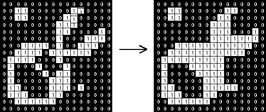
Figure 3. Effect of Morphological Closing on a Binary Image, https://homepages.inf.ed.ac.uk/rbf/HIPR2/close.htm
We initially implemented morphological closing with OpenCV’s erosion and dilation functions, but found that several iterations of each step (5 to 8) were needed to remove noise. This incurred a noticeable time delay, setting the output framerate to only around 5 frames per second. We realized that a more time-efficient method was to use a single iteration with a larger kernel. We found that the laser dot size was maximized while noise artifact size was minimized when the kernel was set to a circle, the same shape as the object of interest (i.e. laser dot). Specifically, we used a 6x6 disc.
Once this was done, we used the findContours function from OpenCV and the grab_contours function from imutils to create an array of all foreground objects (i.e. groups of connected foreground pixels). At this point, we observed that the red and green laser pointer dots were of different sizes consistently -- which was unsurprising given the visible difference in brightness between the two. The green dot had a radius of about 30 pixels, while the red dot had a radius of about 10 pixels. At the same time, there were still a few remaining noise artifacts, though these were much smaller than the dots. This suggested that our next step should be an area-based filter.
We implemented further processing *only* for the foreground object with the maximum area in a given frame, using an approach based on a simple object tracking example [5]. First, we virtually drew the smallest-area circle that enclosed this object (using the cv2.minEnclosingCircle function from OpenCV). Then, if that object ‘s radius was greater than some value (as a subsequent area-based filter), we calculated the coordinates of the centroid of that circle. The coordinates are then remapped to the PIC32’s coordinate space (referenced to the TFT), and then sent via UART to the PIC32 using the serial module in Python.
Hardware Design
Our overall goal in this project was to keep hardware setup minimal, so as to maximize the accessibility of our game to everyone. By the end, the only hardware required were commodity off-the-shelf items: a USB webcam (Logitech QuickCam Pro 9000), a Raspberry Pi 3, a PIC32, a TFT Display, two handheld laser pointers, as well as a document camera connected to a projector (as is commonly found in classrooms). We found that setting up the webcam at a high vantage point facing the screen (e.g. on a tripod) facilitated easy alignment of the projector screen in the webcam’s field of view with minimal distortion of the rectangular region of interest with respect to the computer vision system. However, this requires a long USB cable between the camera and the system set up under the document camera.
One potential improvement to the hardware would be to have a wireless camera instead; this way we would not need to have the long cable. Alternatively, we could have the Pi not just send predator coordinates to the PIC32 but also receive boid coordinates from it and render boids using its onboard HDMI output. A monolithic solution would be to refactor our PIC32 code for a microcontroller with built-in display capabilities. For instance, the RP2040 is such a microcontroller, offering onboard VGA support.
Results
Both our PIC32 boids algorithm and our Python OpenCV code had to meet a variety of performance constraints. Additionally, in our early attempts at two way communication between the PIC and the Raspberry Pi, we also had communication constraints which we were unable to meet due to a variety of challenges that will be discussed further below.
Early Communications Attempts
The most technically challenging aspect of the project was implementing the transfer of boid position data from the PIC to the display medium. The challenge was achieving data transfer at a sufficiently fast rate to render all of the boids, predators, and game scores at an aesthetically pleasing rate (at least 30 fps). We attempted four separate designs for fast communication, listed in the order in which we attempted them:
- Reading serial in Python, rendering the game in Pygame, and using the Pi to drive a projector
- Reading serial in C and writing to a FIFO (Linux named pipe), reading the FIFO in Python and rendering the game in Pygame, and using the Pi to drive a projector
- Reading serial in C++, rendering the game in C++, and using the Pi to drive a projector
- Rendering the game directly on the TFT and using a document camera to send the TFT display to a projector
Communication option 1 suffered from slowness in rendering the game. The PIC, relieved of its duties in driving the TFT, was able to produce data at a high rate (>>30 fps). However, the Python serial library’s readline() method proved incapable of processing the serial transmissions at a rate sufficient to render even 10 fps. We inspected the receive side buffer and found that it grows until overflowing:
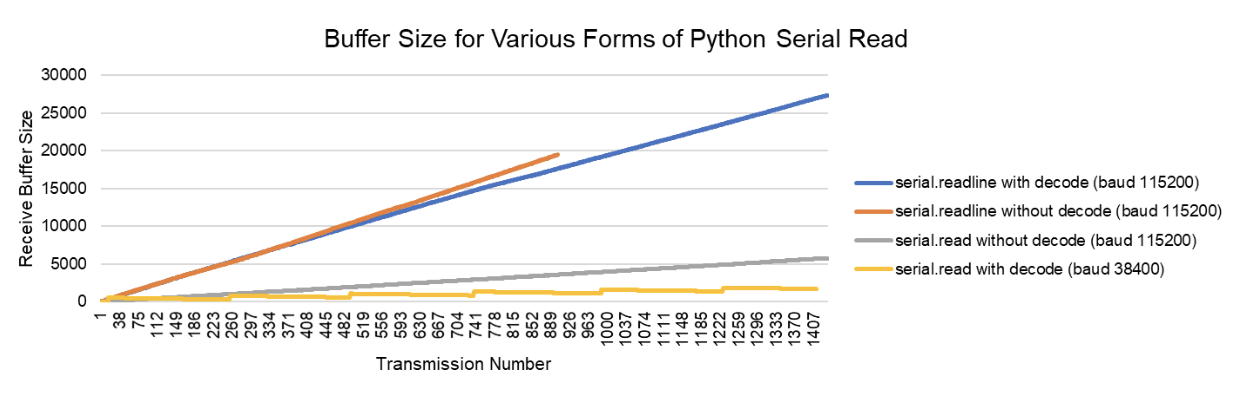
Figure 4. Receive buffer sizes for various forms of Python serial read
As shown in Figure 4, the standard Python serial readline() method resulted in rapid buffer increase. The serial read() method, which reads a single character without waiting for a newline character, is much more lightweight and performs better. We implemented a complete serial read and decode solution with our own buffer management without using the readline() method, but even this failed to perform well:
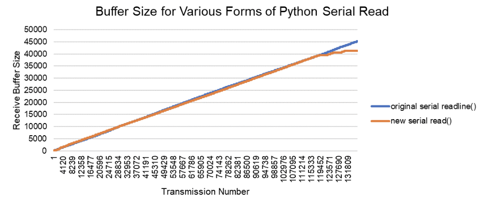
Figure 5. Receive buffer sizes for readline() vs. complete serial read() implementation
We observed another errant feature of our serial read Python code: after an initial period lasting on average half of one second in which serial reads were executed quickly (less than 2 ms between reads), the program entered a state in which one in every 45 serial transmissions took between 60 and 80 ms to read. Observation on an oscilloscope exposed no delays in the serial transmission, so the problem was isolated to the Python side. After experimenting with different baud rates and reducing the PIC transmission rate to no avail, we ultimately found no solution to the problem.
The following video demonstrates the lag in boids rendered using Pygame:
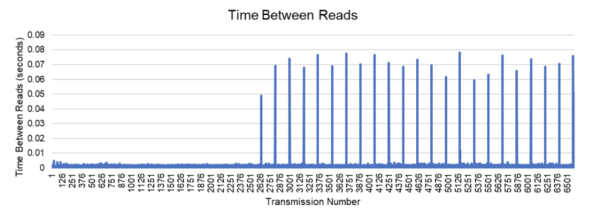
Figure 6. Periodic sharp increases in serial read times in Python
After finding no solution to the problem in Python, we turned to option 2 and implemented a C program to complete serial reads and write the results continuously to a FIFO (first in, first out) buffer in the file system of the Raspberry Pi. The serial reads executed quickly (on the order of 5-6 ms between reads). However, the Python program was unable to read the FIFO quickly, and the Python os.read() method became the new bottleneck. Performance was as poor as a direct Python serial read, and we were only able to render boids at a rate of less than 10 fps.
Upon deciding to eliminate Python from the rendering side of the game entirely, we executed communication option 3 by completing a C++ program to perform serial reads and render boids in a pygame-like window. The program was lightweight and we expected it to improve performance significantly. However, although the performance was marginally better than the Python program, it could only render about 10 boids at a rate over 20 fps. We were targeting 30-50 boids for the final game, and increasing the number of boids to 30 resulted in extremely poor performance.
For option 4, we decided to shift the burden of rendering the game back to the PIC32 and its robust SPI connection to the TFT, thereby trading complexity in high-speed communication for higher demands in program efficiency to accommodate TFT rendering. The PIC could easily handle 30-50 boids at a 30 fps rate for the simple boids algorithm, but adding the demands of the game and the predator control algorithm, as well as increasing the number of boids to 40 in the final version, would ultimately push the PIC to about 30 fps.
C Code Performance
We measured the performance of our game code based on the frame rate we were able to achieve in animation and the communication speeds we were able to achieve over serial. While we experienced significant lag and did not meet our 30 fps animation requirement with the other communication methods described above, once we pivoted to the document camera projection method where we rendered everything on the TFT and applied the same fixed point optimizations as in lab 2, we were able to achieve 30 fps with 40 boids, as well as 2 predators being read through serial, mathematically positioned with lag, and rendered as a circle and a square respectively. This was measured and indicated in the same manner as we used in lab 2, with a red LED indicator on the PIC32 big board that was on when we met our frame rate specifications. This is shown in Figure 7 below. Additionally, once we adopted one way serial communication, we were able to run at a baud rate of 115200 with no issues, indicating that the C program was much faster at serial reading and rendering game objects, since it was a multithreaded implementation.
Figure 7. Red LED on indicating frame rate specs met
Python/CV Code Performance
By the end of the project, we were able to realize a computer vision program that tracked the laser pointer dots in near-realtime, with low latency between movement of the laser pointer and movement of the tracker (enclosing circle plus centroid).
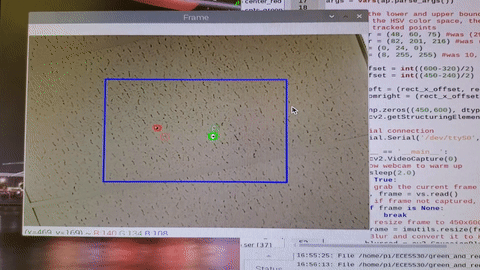
Figure 8. Two-dot tracking using OpenCV
While developing this algorithm, we tried several different sequences of the steps outlined in the Hardware Design section. We found that the first step had to be Gaussian blurring, followed by setting of the color bounds to mask out pixels that were clearly part of the background, in order for the most signal amplification and noise attenuation. Notably, the optimal color bounds that maximized the size of the laser dot while minimizing the size of noise artefacts varied from room to room, based on lighting conditions. As we needed a way to quickly tune the color bounds to the specific environment, we developed a calibration tool, color_detector.py. This tool presented a set of sliders to set upper and lower bounds in the HSV space, with a real-time render of webcam frames masked by those bounds. We had to employ this tool frequently during design and testing.
Tracking gave frequent false positives before adjusting HSV calibration, as shown in the video below:
For the room where we finally performed our demo, Phillips Hall 101, the optimal bounds (in the HSV space) were as follows, in the form of (hue, saturation, value):
greenLower = (40, 50, 75)
greenUpper = (90, 200, 255)
redLower = (0, 95, 42)
redUpper = (6, 255, 255)
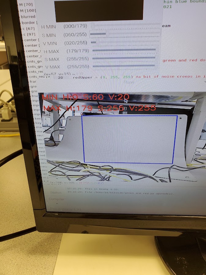
Figure 9. Calibration tool
These were the bounds that maximized the size of the signal (green or red laser dot) while minimizing the size of background noise.
Over the course of the design, we used OpenCV’s built-in functions for the performance-intensive image processing steps (e.g. applying color filtering, finding contours), and we minimized the number of pixel-by-pixel operations throughout image processing (e.g. using large kernel for morphological filtering, limiting pixels by spatial dimensions and color values). Consequently, we found that the computer vision algorithm was actually sending data faster than the PIC32 could process, and so the predator animation was choppy because the PIC32 kept missing predator coordinates updates. Therefore we implemented time delays in two ways. First, we separated the processing for each laser dot. This roughly doubled the time complexity of the computer vision algorithm, since processing originally done on green and red dots together were now done first for the green and then for the red. Second, we implemented a small delay (to further space apart transmission of green and red laser dot coordinates from Pi to PIC32. The optimum delay that provided the smoothest motion on the TFT display was 2 seconds upon program startup, then 1 second for subsequent loops.
The lag in predator updates caused by a discrepancy in transmission vs read speeds is shown in the video below:
After adding in delays on the OpenCV side so that the PIC serial reading could keep up, our performance dramatically improved. The improved performance of the computer vision algorithm was visualized by having it draw visible circles around each laser pointer dot
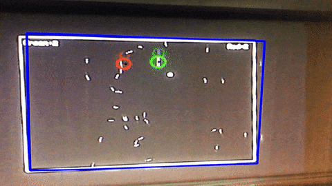
Figure 10. Visualized performance of final computer vision algorithm
After adding in delays on the OpenCV side so that the PIC serial reading could keep up, our performance dramatically improved. Our HSV calibration and vision system were even robust enough that players could stand in the back of Phillips 101 and get reliable predator movement and gameplay! This can be seen in the video below:
Conclusion
Overall, we found that our final project was very successful and we were able to successfully realize our original vision, despite many roadblocks along the way. We learned a great deal about the process of integrating and communicating through multi-device systems, which is especially tricky when devices have different processors and are working in different languages. This is a major challenge in designing and working with embedded systems, and our experience in this proejct will be very valuable to apply to future work in similar fields.
Results vs. Expectations and Future Changes
Overall, we were able to achieve most of our original expectations for this design. Using the document camera projection system as a workaround for two-way communication allowed us to execute our project almost exactly as we had envisioned it in our proposal. Our animation frame rate met the 30 fps standard set in lab 2, and all of our graphics and gameplay elements came together to create a very enjoyable player experience.
Looking back on the project experience, it is clear that two-way communication was our biggest barrier to success. While the document camera projector system was more than sufficient, it would have been helpful to have more backup plans using hardware to achieve projection through the PIC rather than being dependent on an external camera. Late in the design process, we did come across a prior student project that created a VGA connection system for the PIC, but we did not have enough time to buy and put together the necessary hardware at that point. In the future, if the class transitions to use the RP2040 microcontroller instead of the PIC32, this would not be as big of an issue because features like Programmable IO would enable a simpler way to connect to a projector via VGA. Finally, while we did spend significant time and effort in hopes that we would be able to achieve two-way communication, it would have been extremely helpful to our overall project result to have pivoted away from that strategy earlier on in the design process. We were able to add a good amount of gameplay elements to the system in the week that we had to work on it, but with a bit more time we would have been able to come up with many more extensions to the game and would have had a lot more to show for the work we put in to our final product.
Intellectual Property Considerations
This project was developed to be open-source. On the PIC32, our code is based on the Protothreads library, which provides lightweight macros to simplify the process of controlling threads. Protothreads is offered by its creator with a BSD-style license. This is an open-source license that allows both commercial and non-commercial use without restrictions, as long as credit is given in project documentation. On the Raspberry Pi, our computer vision algorithm is based on OpenCV 3.4.6.27, which is also offered with a BSD license.
Ethical Considerations
This project was designed with accessibility in mind, particularly for those with red-green colorblindness. Although a person with red-green colorblindness may not be able to differentiate the two lasers by their colors, the two lasers can be told apart by their brightness. Since the green laser is significantly brighter than the red laser, any person unable to identify the colors can differentiate the size of the points on the screen. In addition, the predator positions are denoted by two different shapes: a circle for green and a square for red. All other components of the game are projected in black and white. An additional ethical consideration is that the computer vision technology used in this project can also be used in the unethical application of surveillance through facial recognition. Since this project only tracks objects by color, there is no risk of the project being used for unethical activities.
Safety Considerations
For safety, all spectators are required to stand behind the players to avoid accidental eye exposure to the lasers. All of the laser pointers used in this game are Class 3A or lower, meaning they are legal and safe for use without eye protection. The green laser is Class 3A, denoting an output power which does not exceed 5 mW and a beam power density which does not exceed 2.5 mW/cm2. Class 3A lasers can be damaging to the retina only after over two minutes of direct exposure. The red laser is Class 2, indicating an output power of less than 1 mW. Class 2 lasers will not cause retinal damage. Children should not be allowed to play the game due to the heightened risk of exposing spectators to the lasers.
Legal Considerations
According to the United States Food and Drug Administration, lasers for pointing or demonstration use must not exceed 5 mW of output power (the limit for Class 3A laser pointers). All of the laser pointers used in this project are Class 3A or lower and are therefore compliant with federal regulations for their use in this game.
Work Distribution
Claire worked on the C code running on the PIC32, including updates to support 2 predators over serial read, updates to the boids animation to reflect predators eating them and scoring points, and direct digital synthesis sound effects. She worked with Alec and Shreyas throughout the communication debugging process. She also implemented the C++ aspects of communication option 3, including the final test implementation with the SFML bouncing ball library and WiringPi serial read. She also collaborated with Alec on coding the TFT game elements to optimize the gameplay experience, such as the scoring and boundary displays, the winning player screen, as well as other attempts at gameplay extensions like a start screen which did not make it into the final implementation.
Shreyas developed the computer vision system, consisting of Python scripts running on a Raspberry Pi. The system consisted of several stages: video manipulation, image processing, object detection, and centroid estimation. He wrote the code for each stage iteratively, optimizing the sequence and parameters of operations to produce reliable and accurate tracking of two laser dots simultaneously in a range of lighting conditions. He also developed a calibration program that allows quick tuning of image processing parameters to specific indoor environments. In addition, he collaborated with Claire and Alec on developing the various iterations of serial communication on the Pi, and was responsible for color tuning and computer vision setup during full system testing in various classrooms.
Alec wrote the code for the early attempts to render boids in pygame and incorporated the “laggy predator” design. He worked to debug the serial read problems, implementing several versions of serial read in Python including versions with manual buffer management in the effort to circumvent problems with the readline() method. Alec collected data to troubleshoot the communication problem and produced all of the measurements and plots shown in the Early Communications Attempts section. He worked with Shreyas and Claire to build and test communication options 2 and 3, and he assembled the breadboard and wood block mount for the PIC and the Pi and wired the breadboard for serial communication. He collaborated with Claire to write the game code and optimize the game performance.
Appendix
Appendix A: Permissions
The group approves this report for inclusion on the course website.
The group approves the video for inclusion on the course YouTube channel.
Appendix B: Commented Code
The complete project source code is hosted on GitLab: https://github.com/crcaplan/ece5730/tree/main/final_project
C program with comments is given below (extended from TFT_animation_Accum_BRL4.c):
/* * File: Test of compiler fixed point * Author: Bruce Land * Adapted from: * main.c by * Author: Syed Tahmid Mahbub * Target PIC: PIC32MX250F128B */ //////////////////////////////////// // clock AND protoThreads configure #include "config_1_3_2.h" // threading library #include "pt_cornell_1_3_2.h" //////////////////////////////////// // graphics libraries #include "tft_master.h" #include "tft_gfx.h" // need for rand function #include <stdlib.h> // fixed point types #include <stdfix.h> //need for sqrt #include <math.h> //need for memcpy #include <string.h> //need for sleep #include<stdio.h> //////////////////////////////////// /* Demo code for interfacing TFT (ILI9340 controller) to PIC32 * The library has been modified from a similar Adafruit library */ // Adafruit data: /*************************************************** This is an example sketch for the Adafruit 2.2" SPI display. This library works with the Adafruit 2.2" TFT Breakout w/SD card ----> http://www.adafruit.com/products/1480 Check out the links above for our tutorials and wiring diagrams These displays use SPI to communicate, 4 or 5 pins are required to interface (RST is optional) Adafruit invests time and resources providing this open source code, please support Adafruit and open-source hardware by purchasing products from Adafruit! Written by Limor Fried/Ladyada for Adafruit Industries. MIT license, all text above must be included in any redistribution ****************************************************/ // DDS setup pulled from lab 1 // lock out timer interrupt during spi comm to port expander // This is necessary if you use the SPI2 channel in an ISR #define start_spi2_critical_section INTEnable(INT_T2, 0); #define end_spi2_critical_section INTEnable(INT_T2, 1); // some precise, fixed, short delays // to use for extending pulse durations on the keypad // if behavior is erratic #define NOP asm("nop"); // 20 cycles #define wait20 NOP;NOP;NOP;NOP;NOP;NOP;NOP;NOP;NOP;NOP;NOP;NOP;NOP;NOP;NOP;NOP;NOP;NOP;NOP;NOP; // 40 cycles #define wait40 wait20;wait20; // define fs for use in DDS algorithm float two_32_fs = 4294967296.0 / 44000.0; #define two32fs two_32_fs // string buffer for TFT printing char buffer[60]; // define boid struct typedef struct { _Accum x; // x position _Accum y; // y position _Accum vx; // x velocity _Accum vy; // y velocity int eaten; // eaten flag } boid_t; // boid control values, can be edited // original suggested values shown in comments _Accum turnfactor = 0.2; //0.2 _Accum visualrange = 20; // 20 int protectedrange = 2; //2 _Accum centeringfactor = 0.0005; //0.0005 _Accum avoidfactor = 0.05; // 0.05 _Accum matchingfactor = 0.05; // 0.05 int maxspeed = 3; //3 int maxspeed_sq = 9; //9 int minspeed = 2; //2 int minspeed_sq = 4; //4 int topmargin = 50; //50 int bottommargin = 50; //50 int leftmargin = 50; //50 int rightmargin = 50; //50 float predspeedfactor = 0.25; // 0.15 int predmaxspeed = 100; // 0.03 //Predator control values _Accum predatorturnfactor = 0.4; //0.4 _Accum predatorrange = 50; // 50 //Predator eating control _Accum deathrange = 30; // 30 // === outputs from python handler ============================================= // signals from the python handler thread to other threads // These will be used with the prototreads PT_YIELD_UNTIL(pt, condition); // to act as semaphores to the processing threads char new_string = 0; char new_button = 0; char new_toggle = 0; char new_slider = 0; char new_list = 0 ; char new_radio = 0 ; // identifiers and values of controls // current button char button_id, button_value ; // current toggle switch/ check box char toggle_id, toggle_value ; // current radio-group ID and button-member ID char radio_group_id, radio_member_id ; // current slider int slider_id; float slider_value ; // value could be large // current listbox int list_id, list_value ; // current string char receive_string[64]; // system 1 second interval tick int sys_time_seconds ; // === Define all variables and constants for DDS algorithm ========== // Audio DAC ISR // A-channel, 1x, active #define DAC_config_chan_A 0b0011000000000000 // B-channel, 1x, active #define DAC_config_chan_B 0b1011000000000000 // audio sample frequency #define Fs 44000.0 // need this constant for setting DDS frequency #define two32 4294967296.0 // 2^32 // sine lookup table for DDS #define sine_table_size 256 volatile _Accum sine_table[sine_table_size] ; // phase accumulator for DDS volatile unsigned int DDS_phase ; // phase increment to set the frequency DDS_increment = Fout*two32/Fs // For A above middle C DDS_increment = = 42949673 = 440.0*two32/Fs //#define Fout 440.0 //volatile unsigned int DDS_increment = Fout*two32/Fs ; //42949673 ; // waveform amplitude volatile _Accum max_amplitude=2000; // waveform amplitude envelope parameters // rise/fall time envelope 44 kHz samples volatile unsigned int attack_time=500, decay_time=500, sustain_time=1000 ; // 0<= current_amplitude < 2048 volatile _Accum current_amplitude ; // amplitude change per sample during attack and decay // no change during sustain volatile _Accum attack_inc, decay_inc ; volatile unsigned int DAC_data_A, DAC_data_B ; // output values volatile SpiChannel spiChn = SPI_CHANNEL2 ; // the SPI channel to use volatile int spiClkDiv = 4 ; // 10 MHz max speed for port expander!! // interrupt ticks since beginning of song or note volatile unsigned int song_time, note_time ; // predefined constant to minimize floating point calculations float pi_max_amp = 3.1415926535 / 5720.0; #define pimaxamp pi_max_amp volatile float Fout = 440.0; volatile int sound = -1; volatile unsigned int DDS_increment; unsigned int isr_time; volatile float note_sec; // === DDS interrupt service routine ================================ void __ISR(_TIMER_2_VECTOR, ipl2) Timer2Handler(void) { // set different frequency for each predator's eating sound switch (sound) { case 1: // player 1 sound Fout = 330; break; case 2: // player 2 sound Fout = 440; break; default: Fout = 0; break; } // DDS increment to advance phase DDS_increment = (unsigned int) (Fout * two32fs); int junk; mT2ClearIntFlag(); // generate sinewave // advance the phase DDS_phase += DDS_increment ; //DAC_data += 1 & 0xfff ; // low frequency ramp DAC_data_A = (int)(current_amplitude*sine_table[DDS_phase>>24]) + 2048 ; // for testing sine_table[DDS_phase>>24] // update amplitude envelope if (note_time < (attack_time + decay_time + sustain_time)){ current_amplitude = (note_time <= attack_time)? current_amplitude + attack_inc : (note_time <= attack_time + sustain_time)? current_amplitude: current_amplitude - decay_inc ; } else { current_amplitude = 0 ; } // test for ready while (TxBufFullSPI2()); // reset spi mode to avoid conflict with expander SPI_Mode16(); // DAC-A CS low to start transaction mPORTBClearBits(BIT_4); // start transaction // write to spi2 WriteSPI2(DAC_config_chan_A | (DAC_data_A & 0xfff) ); // fold a couple of timer updates into the transmit time song_time++ ; // cap note time at 6000 to shorten tone's play time if (note_time <= 6000) { note_time++ ; } // test for done while (SPI2STATbits.SPIBUSY); // wait for end of transaction // MUST read to clear buffer for port expander elsewhere in code junk = ReadSPI2(); // CS high mPORTBSetBits(BIT_4); // end transaction isr_time = ReadTimer2(); } //=== Timer Thread ================================================= //update a 1 second tick counter static PT_THREAD (protothread_timer(struct pt *pt)) { PT_BEGIN(pt); while(1) { // yield time 1 second PT_YIELD_TIME_msec(1000) ; sys_time_seconds++ ; // NEVER exit while } // END WHILE(1) PT_END(pt); } // timer thread // === Animation Thread ============================================= // define fixed <--> float conversion macros #define float2Accum(a) ((_Accum)(a)) #define Accum2float(a) ((float)(a)) #define int2Accum(a) ((_Accum)(a)) #define Accum2int(a) ((int)(a)) // define gameplay constants #define NUM_BOIDS 40 #define NUM_PREDATORS 2 #define SCREEN_WIDTH_X 320 #define SCREEN_HEIGHT_Y 240 #define PREDATOR_SIZE 2 // initialize all fixed point boid variables _Accum xpos_avg; _Accum ypos_avg; _Accum xvel_avg; _Accum yvel_avg; _Accum neighboring_boids; _Accum close_dx; _Accum close_dy; _Accum speed; _Accum speed_sq; _Accum predator_speed; _Accum predator_speed_sq; // initialize all fixed point predator variables _Accum predator_dy; _Accum predator_dx; _Accum num_predators; // initialize boid and predator arrays boid_t boid_array[NUM_BOIDS]; boid_t predator_array[NUM_PREDATORS]; // iteration variables for loops int i=0; int j=0; int k=0; int h=0; // initialize player scores int score1 = 0; int score2 = 0; // initial predator positions int pred_x=100; int pred_y=100; // flag to alternate rendering game borders and scores // optimized because not necessary to draw all of them each time int score_draw = 0; static PT_THREAD (protothread_anim(struct pt *pt)) { PT_BEGIN(pt); // draw 4 lines around the border of the TFT tft_drawLine(0, 0, 320, 0, ILI9340_WHITE); tft_drawLine(319, 0, 319, 240, ILI9340_WHITE); tft_drawLine(0, 239, 320, 239, ILI9340_WHITE); tft_drawLine(0, 0, 0, 240, ILI9340_WHITE); // randomly initialize elements into boid and predator arrays int idxB; int idxP; static _Accum Accum_rand_x, Accum_rand_y, Accum_rand_vx, Accum_rand_vy; for (idxB = 0; idxB < NUM_BOIDS; idxB++){ srand(idxB); Accum_rand_x = ((_Accum)(rand() & 0xffff) >> 8) - 16; Accum_rand_y = ((_Accum)(rand() & 0xffff) >> 7) - 192; Accum_rand_vx = ((_Accum)(rand() & 0xffff) >> 16) + 2; Accum_rand_vy = ((_Accum)(rand() & 0xffff) >> 16) + 2; boid_t entry_boid = {.x = Accum_rand_x, .y = Accum_rand_y, .vx = Accum_rand_vx, .vy = Accum_rand_vy, .eaten=0}; boid_array[idxB] = entry_boid; } for (idxP = 0; idxP < NUM_PREDATORS; idxP++){ srand(idxP); Accum_rand_x = ((_Accum)(rand() & 0xffff) >> 8) - 16; Accum_rand_y = ((_Accum)(rand() & 0xffff) >> 7) - 192; Accum_rand_vx = ((_Accum)(rand() & 0xffff) >> 16) + 2; Accum_rand_vy = ((_Accum)(rand() & 0xffff) >> 16) + 2; } boid_t predator_boid = {.x = 100, .y = 100, .vx = Accum_rand_vx, .vy = Accum_rand_vy, .eaten=0}; boid_t predator_boid2 = {.x = 200, .y = 200, .vx = Accum_rand_vx, .vy = Accum_rand_vy, .eaten=0}; predator_array[0] = predator_boid; predator_array[1] = predator_boid2; // initialize boid and predator to be pulled from array each iteration static boid_t boid; static boid_t predator; // set up LED to indicate if we are meeting frame rate mPORTASetBits(BIT_0); //Clear bits to ensure light is off. mPORTASetPinsDigitalOut(BIT_0); //Set port as output while(1) { // track time in animation loop to calculate frame rate unsigned int begin_time = PT_GET_TIME(); // increase predator range as more boids are eaten // makes game more difficult near the end if(score1+score2>20){ predatorrange = 55; }else if(score1+score2>30){ predatorrange = 60; } for(i = 0; i<NUM_BOIDS; i++){ // get copy of boid from boid array boid = boid_array[i]; // if boid has not been eaten if(boid.eaten < 4){ //erase boid pixel tft_drawPixel(Accum2int(boid.x), Accum2int(boid.y), ILI9340_BLACK); //x, y, radius, color // zero all accumulator variables xpos_avg = 0; ypos_avg = 0; xvel_avg = 0; yvel_avg = 0; neighboring_boids = 0; close_dx = 0; close_dy = 0; num_predators = 0; predator_dx = 0; predator_dy = 0; // loop to determine motion based on neighboring boids for (j=(i+1); j<NUM_BOIDS; j++){ // get copy of neighboring boid from array boid_t otherboid = boid_array[j]; // if neighbor hasn't been eaten if(otherboid.eaten == 0){ //compute differences in x and y coordinates _Accum dx = boid.x - otherboid.x; _Accum dy = boid.y - otherboid.y; // are both of those differences less than the visual range? if ((abs(dx)<visualrange) && (abs(dy)<visualrange)){ // if so, calculate the squared distance _Accum squared_distance = dx*dx + dy*dy; // is squared distance less than protected range? if(squared_distance < (protectedrange*protectedrange)){ // if so, calculate difference in x,y coordinates to nearfield boid close_dx += dx; close_dy += dy; } // if not in protected range, is the boid in the visual range? else if(squared_distance < (visualrange*visualrange)){ //add otherboid's x,y coordinates and x,y vel to accumulator vars xpos_avg += otherboid.x; ypos_avg += otherboid.y; xvel_avg += otherboid.vx; yvel_avg += otherboid.vy; // increment number of boids within visual range neighboring_boids += 1; } } } } // loop to determine motion based on nearby predators for(k=0;k<NUM_PREDATORS;k++){ predator = predator_array[k]; // Compute the differences in x and y coordinates _Accum dx = boid.x - predator.x; _Accum dy = boid.y - predator.y; // Are both those differences less than predatory range if(abs(dx)<predatorrange && abs(dy) < predatorrange){ //If so, calculate squared distance to predator _Accum squaredpredatordistance = dx*dx + dy*dy; //Is the squared distance less than predatory range squared if(squaredpredatordistance<predatorrange*predatorrange){ //If so, accumulate the differences in x/y to the predator predator_dx += boid.x - predator.x; predator_dy += boid.y - predator.y; //Increment the number of predators in the boid's predatory range num_predators += 1; } } // If there were any predators in the predatory range, turn away if(num_predators>0){ if(predator_dy>0) boid.vy += predatorturnfactor; if(predator_dy<0) boid.vy -= predatorturnfactor; if(predator_dx>0) boid.vx += predatorturnfactor; if(predator_dx<0) boid.vx -= predatorturnfactor; } } // loop to determine if boid should be eaten for(h=0;h<NUM_PREDATORS;h++){ // get copy of predator from array predator = predator_array[h]; // Compute the differences in x and y coordinates _Accum dx = boid.x - predator.x; _Accum dy = boid.y - predator.y; // Are both those differences less than death range if(abs(dx)<deathrange && abs(dy) < deathrange){ //If so, calculate squared distance to predator _Accum squaredpredatordistance = dx*dx + dy*dy; //Is the squared distance less than death range squared if(squaredpredatordistance<deathrange*deathrange){ // if boid has not been eaten yet if(boid.eaten == 0){ // set 'eaten' flag on boid boid.eaten = 1; // increment scoring for the predator who ate it // trigger DDS interrupt to play sound effect if(h == 0){ score1 += 1; sound = 1; note_time = 0; }else{ score2 += 1; sound = 2; note_time = 0; } // if all boids have been eaten, display end screen // show winner and final score if(score1+score2 >= NUM_BOIDS){ // player 1 wins if(score1 > score2){ tft_fillScreen(ILI9340_GREEN); // print msg tft_setCursor(70, 100); tft_setTextColor(ILI9340_WHITE); tft_setTextSize(3); sprintf(buffer,"Green Wins!"); tft_writeString(buffer); // print score tft_setCursor(100, 130); tft_setTextColor(ILI9340_WHITE); tft_setTextSize(3); sprintf(buffer,"%d - %d", score1, score2); tft_writeString(buffer); while(1); // stay on end screen until reset // player 2 wins }else if (score2 > score1){ tft_fillScreen(ILI9340_RED); // print msg tft_setCursor(80, 100); tft_setTextColor(ILI9340_WHITE); tft_setTextSize(3); sprintf(buffer,"Red Wins!"); tft_writeString(buffer); // print score tft_setCursor(100, 130); tft_setTextColor(ILI9340_WHITE); tft_setTextSize(3); sprintf(buffer,"%d - %d", score2, score1); tft_writeString(buffer); while(1); // stay on end screen until reset } } } } } } //if there were any boids in the visual range if(neighboring_boids > 0){ // divide accumulator variables by number of boids in visual range _Accum neighbor_factor = 1/neighboring_boids; xpos_avg = xpos_avg*neighbor_factor; ypos_avg = ypos_avg*neighbor_factor; xvel_avg = xvel_avg*neighbor_factor; yvel_avg = yvel_avg*neighbor_factor; // add the centering/matching contributions to velocity boid.vx += (xpos_avg - boid.x)*centeringfactor + (xvel_avg - boid.vx)*matchingfactor; boid.vy += (ypos_avg - boid.y)*centeringfactor + (yvel_avg - boid.vy)*matchingfactor; } // add the avoidance contribution to velocity boid.vx += close_dx*avoidfactor; boid.vy += close_dy*avoidfactor; //if the boid is near an edge, make it turn by turn factor if(boid.y > SCREEN_HEIGHT_Y - topmargin){ boid.vy = boid.vy - turnfactor; } if(boid.x > SCREEN_WIDTH_X - rightmargin){ boid.vx = boid.vx - turnfactor; } if(boid.x < leftmargin){ boid.vx = boid.vx + turnfactor; } if(boid.y < bottommargin){ boid.vy = boid.vy + turnfactor; } // Original logic based on lab pseudocode //calculate the boid's speed and predator's speed speed = sqrt(boid.vx*boid.vx + boid.vy*boid.vy); _Accum speed_factor_min = minspeed/speed; _Accum speed_factor_max = maxspeed/speed; //enforce min and max speeds if (speed < minspeed){ boid.vx = boid.vx*speed_factor_min; boid.vy = boid.vy*speed_factor_min; } if (speed > maxspeed){ boid.vx = boid.vx*speed_factor_max; boid.vy = boid.vy*speed_factor_max; } // update boid position if it hasn't been eaten if(boid.eaten == 0){ boid.x = boid.x + boid.vx; boid.y = boid.y + boid.vy; } // Draw boid pixel if it hasn't been eaten // if boid has been eaten, follow sequence of explosion animation if(boid.eaten == 0){ tft_drawPixel(Accum2int(boid.x), Accum2int(boid.y), ILI9340_WHITE); }else if(boid.eaten == 1){ tft_fillCircle(Accum2int(boid.x), Accum2int(boid.y), 2, ILI9340_YELLOW); boid.eaten += 1; }else if(boid.eaten == 2){ tft_fillCircle(Accum2int(boid.x), Accum2int(boid.y), 2, ILI9340_YELLOW); boid.eaten += 1; }else if(boid.eaten == 3){ tft_fillCircle(Accum2int(boid.x), Accum2int(boid.y), 2, ILI9340_BLACK); boid.eaten += 1; }else{ tft_drawPixel(Accum2int(boid.x), Accum2int(boid.y), ILI9340_BLACK); } // save updated boid struct back into boid array boid_array[i] = boid; } } // rotate between redrawing half of the game elements // in case boids have flown over them if(score_draw == 0){ // player 1 score tft_setCursor(5, 7); tft_fillRoundRect(38,5, 15, 9, 1, ILI9340_BLACK); tft_setTextColor(ILI9340_WHITE); tft_setTextSize(1); sprintf(buffer,"Green:%d", score1); tft_writeString(buffer); score_draw = 1; //lines tft_drawLine(0, 0, 320, 0, ILI9340_WHITE); tft_drawLine(319, 0, 319, 240, ILI9340_WHITE); }else if(score_draw == 1){ // player 2 score tft_setCursor(280, 7); tft_fillRoundRect(302,5, 15, 9, 1, ILI9340_BLACK); tft_setTextColor(ILI9340_WHITE); tft_setTextSize(1); sprintf(buffer,"Red:%d", score2); tft_writeString(buffer); score_draw = 0; //lines tft_drawLine(0, 239, 320, 239, ILI9340_WHITE); tft_drawLine(0, 0, 0, 240, ILI9340_WHITE); } //find frame rate _Accum frame_period = (PT_GET_TIME() - begin_time); PT_YIELD_TIME_msec(33 - frame_period); // if we are meeting frame rate spec, turn LED on if(frame_period > 33){ mPORTAClearBits(BIT_0); } else{ mPORTASetBits(BIT_0); } // NEVER exit while } // END WHILE(1) PT_END(pt); } // end animation thread // === string input thread ===================================================== // process text from python static PT_THREAD (protothread_python_string(struct pt *pt)) { PT_BEGIN(pt); // initialize variables to handle predator static boid_t predator; static int laser_x,laser_y,posn_diff,move_x,move_y,pred_x,pred_y,pred_id,pred_speed; while(1){ // wait for a new string from Python and read it in PT_YIELD_UNTIL(pt, new_string==1); new_string = 0; sscanf(receive_string, "%d,%d,%d", &pred_id, &laser_x, &laser_y); // get predator from array using received ID value predator = predator_array[pred_id]; // erase the appropriate predator if(pred_id == 0){ tft_fillCircle(Accum2int(predator.x), Accum2int(predator.y), PREDATOR_SIZE, ILI9340_BLACK); }else{ tft_fillRect(Accum2int(predator.x), Accum2int(predator.y), 4, 4, ILI9340_BLACK); } // determine new coordinates through lagging mechanism move_x = (laser_x-predator.x)*predspeedfactor; move_y = (laser_y-predator.y)*predspeedfactor; if(move_x > predmaxspeed) { move_x = predmaxspeed; } if(move_y > predmaxspeed) { move_y = predmaxspeed; } // set new coordinates predator.x = (int) (predator.x + move_x); predator.y = (int) (predator.y + move_y); // Draw predator (circle or square depending on which player) if(pred_id == 0){ //printf("%d,%d,%d\n", h+NUM_BOIDS, Accum2int(predator.x), Accum2int(predator.y)); tft_fillCircle(Accum2int(predator.x), Accum2int(predator.y), PREDATOR_SIZE, ILI9340_WHITE); }else{ //printf("%d,%d,%d\n", h+NUM_BOIDS, Accum2int(predator.x), Accum2int(predator.y)); tft_fillRect(Accum2int(predator.x), Accum2int(predator.y), 4, 4, ILI9340_WHITE); } // save updated predator struct back into array predator_array[pred_id] = predator; } // END WHILE(1) PT_END(pt); } // end python_string // === Python serial thread (pulled from lab 2)============================================ // you should not need to change this thread UNLESS you add new control types static PT_THREAD (protothread_serial(struct pt *pt)) { PT_BEGIN(pt); static char junk; // // while(1){ // There is no YIELD in this loop because there are // YIELDS in the spawned threads that determine the // execution rate while WAITING for machine input // ============================================= // NOTE!! -- to use serial spawned functions // you MUST edit config_1_3_2 to // (1) uncomment the line -- #define use_uart_serial // (2) SET the baud rate to match the PC terminal // ============================================= // now wait for machine input from python // Terminate on the usual <enter key> PT_terminate_char = '\r' ; PT_terminate_count = 0 ; PT_terminate_time = 0 ; // note that there will NO visual feedback using the following function PT_SPAWN(pt, &pt_input, PT_GetMachineBuffer(&pt_input) ); // Parse the string from Python // There can be toggle switch, button, slider, and string events // string from python input line if (PT_term_buffer[0]=='$'){ // signal parsing thread new_string = 1; // output to thread which parses the string // while striping off the '$' strcpy(receive_string, PT_term_buffer+1); } } // END WHILE(1) PT_END(pt); } // end python serial // === Main ====================================================== void main(void) { ANSELA = 0; ANSELB = 0; // === DDS setup code ========================== // set up DAC on big board // timer interrupt ////////////////////////// // Set up timer2 on, interrupts, internal clock, prescalar 1, toggle rate // at 40 MHz PB clock // 40,000,000/Fs = 909 : since timer is zero-based, set to 908 OpenTimer2(T2_ON | T2_SOURCE_INT | T2_PS_1_1, 908); // set up the timer interrupt with a priority of 2 ConfigIntTimer2(T2_INT_ON | T2_INT_PRIOR_2); mT2ClearIntFlag(); // and clear the interrupt flag // SCK2 is pin 26 // SDO2 (MOSI) is in PPS output group 2, could be connected to RB5 which is pin 14 PPSOutput(2, RPB5, SDO2); // control CS for DAC mPORTBSetPinsDigitalOut(BIT_4); mPORTBSetBits(BIT_4); // divide Fpb by 2, configure the I/O ports. Not using SS in this example // 16 bit transfer CKP=1 CKE=1 // possibles SPI_OPEN_CKP_HIGH; SPI_OPEN_SMP_END; SPI_OPEN_CKE_REV // For any given peripherial, you will need to match these // clk divider set to 4 for 10 MHz SpiChnOpen(SPI_CHANNEL2, SPI_OPEN_ON | SPI_OPEN_MODE16 | SPI_OPEN_MSTEN | SPI_OPEN_CKE_REV , 4); // end DAC setup // // build the sine lookup table // scaled to produce values between 0 and 4096 int i; for (i = 0; i < sine_table_size; i++){ sine_table[i] = (_Accum)(sin((float)i*6.283/(float)sine_table_size)); } // build the amplitude envelope parameters // bow parameters range check if (attack_time < 1) attack_time = 1; if (decay_time < 1) decay_time = 1; if (sustain_time < 1) sustain_time = 1; // set up increments for calculating bow envelope attack_inc = max_amplitude/(_Accum)attack_time ; decay_inc = max_amplitude/(_Accum)decay_time ; // === setup system wide interrupts ======== INTEnableSystemMultiVectoredInt(); // === TFT setup ============================ // init the display in main since more than one thread uses it. // NOTE that this init assumes SPI channel 1 connections tft_init_hw(); tft_begin(); tft_fillScreen(ILI9340_BLACK); //set horizontal display, 320x240 tft_setRotation(3); // === config threads ========== // turns OFF UART support and debugger pin, unless defines are set PT_setup(); pt_add(protothread_serial, 0); pt_add(protothread_python_string, 0); pt_add(protothread_timer, 0); pt_add(protothread_anim, 0); // init the threads PT_INIT(&pt_sched) ; // === identify the threads to the scheduler ===== // add the thread function pointers to be scheduled // --- Two parameters: function_name and rate. --- // rate=0 fastest, rate=1 half, rate=2 quarter, rate=3 eighth, rate=4 sixteenth, // rate=5 or greater DISABLE thread! // seed random color srand(2); // round-robin scheduler for threads pt_sched_method = SCHED_ROUND_ROBIN ; // === scheduler thread ======================= // scheduler never exits PT_SCHEDULE(protothread_sched(&pt_sched)); // === end ======================================================
Python/OpenCV computer vision program with comments is given below (green_and_red_2.py)
'''
Simultaneous tracking of two laser pointers (red and green) with serial output
Place Region of Interest (ROI) within blue bounding box
by Shreyas Renganathan, December 2021
'''
# import the necessary packages
from imutils.video import VideoStream
import numpy as np
import cv2
import imutils
import time
import serial

# define lower and upper bounds of green and red dots
greenLower = (40, 50, 75)
greenUpper = (90, 200, 255)
redLower = (0, 95, 42) #was 82
redUpper = (6, 255, 255) # was 10,255,255

rect_x_offset = int((600-320)/2)
rect_y_offset = int((450-240)/2)

rect_topleft = (rect_x_offset, rect_y_offset)
rect_bottomright = (rect_x_offset+320, rect_y_offset+240)

border = np.zeros((450,600), dtype="uint8")
kernel = cv2.getStructuringElement(cv2.MORPH_ELLIPSE, (6, 6))

#open serial connection
ser = serial.Serial('/dev/ttyS0', 38400, timeout=0.001)
delay = 5

if __name__ == '__main__':
	vs = cv2.VideoCapture(0)
	# allow webcam to warm up
	time.sleep(2.0)
	while True:
		# Read a frame
		_, frame = vs.read()
		# If frame not captured, exit
		if frame is None:
			break
		# Resize frame to 450x600 for quicker turnaround
		frame = imutils.resize(frame, width=600)
		# Blur and convert it to HSV
		blurred = cv2.GaussianBlur(frame, (11, 11), 0)
		hsv = cv2.cvtColor(blurred, cv2.COLOR_BGR2HSV)
		# Construct mask for green passband
		mask_green = cv2.inRange(hsv, greenLower, greenUpper)
		# Draw ROI and mask out border outside ROI
		cv2.rectangle(frame, pt1=rect_topleft, pt2=rect_bottomright, color=(255,0,0), thickness=2)
		cv2.rectangle(border, rect_topleft, rect_bottomright, 255, thickness=-1)
		result_green = cv2.bitwise_and(mask_green, mask_green, mask=border)
		# Isolate laser dot in each mask by morphological closing
		result_green = cv2.morphologyEx(result_green, cv2.MORPH_CLOSE, kernel)
		# Find all blobs in green mask
		cnts_green = cv2.findContours(result_green.copy(), cv2.RETR_EXTERNAL, cv2.CHAIN_APPROX_SIMPLE)
		cnts_green = imutils.grab_contours(cnts_green)
		center_green = None
		# Only proceed if at least one green blob was found
		if len(cnts_green) > 0:
			# Find largest blob on green mask
			c = max(cnts_green, key=cv2.contourArea)
			# Calculate smallest enclosing circle and centroid for it
			((x, y), radius) = cv2.minEnclosingCircle(c)
			M = cv2.moments(c)
			# Proceed only if a large blob exists (green laser dot is present)
			if (M["m00"]!=0):
				center = (int(M["m10"] / M["m00"]), int(M["m01"] / M["m00"]))
				# Only proceed if blob circle radius greater than some size
				# and blob within ROI
				if radius > 3 and x >= rect_x_offset and x <= rect_x_offset + 320 and y >= rect_y_offset and y <= rect_y_offset + 240:
					# Draw circle and centroid for the large blob
					cv2.circle(frame, (int(x), int(y)), int(radius), (0, 255, 0), 2)
					cv2.circle(frame, center, 2, (0, 0, 0), -1)
					x_in_box = x - rect_x_offset
					y_in_box = y - rect_y_offset
					input_state_green = '0'+','+str(int(x_in_box))+','+str(int(y_in_box)) #idx 0 is green
					# add <cr> for PIC
					input_state_green_final = '$' + input_state_green + '\r'
					#print(input_state_green_final)
					# send to PIC protothreads
					ser.write((input_state_green_final).encode())
		if delay > 2: #was 3
			delay=delay-1
		time.sleep(float(delay)/100.0)
		# Construct mask for red passband
		mask_red = cv2.inRange(hsv, redLower, redUpper)
		# Draw ROI and mask out border outside ROI
		result_red = cv2.bitwise_and(mask_red, mask_red, mask=border)
		# Isolate laser dot in each mask by morphological closing
		result_red = cv2.morphologyEx(result_red, cv2.MORPH_CLOSE, kernel)
		# Find all blobs in red mask
		cnts_red = cv2.findContours(result_red.copy(), cv2.RETR_EXTERNAL, cv2.CHAIN_APPROX_SIMPLE)
		cnts_red = imutils.grab_contours(cnts_red)
		center_red = None
		# Only proceed if at least one red blob was found
		if len(cnts_red) > 0:
			# Find largest blob on red mask
			c = max(cnts_red, key=cv2.contourArea)
			# Calculate smallest enclosing circle and centroid for it
			((x, y), radius) = cv2.minEnclosingCircle(c)
			M = cv2.moments(c)
			# Proceed only if a large blob exists (red laser dot is present)
			if (M["m00"]!=0):
				center = (int(M["m10"] / M["m00"]), int(M["m01"] / M["m00"]))
				# Only proceed if blob circle radius greater than some size
				# and blob within ROI
				if radius > 3 and x >= rect_x_offset and x <= rect_x_offset + 320 and y >= rect_y_offset and y <= rect_y_offset + 240:
					# Draw circle and centroid for the large blob
					cv2.circle(frame, (int(x), int(y)), int(radius), (0, 0, 255), 2)
					cv2.circle(frame, center, 2, (0, 0, 0), -1)
					x_in_box = x - rect_x_offset
					y_in_box = y - rect_y_offset
					input_state_red = '1'+','+str(int(x_in_box))+','+str(int(y_in_box)) #idx 1 is red
					# add <cr> for PIC
					input_state_red_final = '$' + input_state_red + '\r'
					#print(input_state_red_final)
					# send to PIC protothreads
					ser.write((input_state_red_final).encode())
		# Display the frame on screen
		cv2.imshow("Frame", frame)
		key = cv2.waitKey(1) & 0xFF
		# if 'q' or 'ESC' key is pressed, end main loop
		if key == ord("q") or key == 27:
			break

# Stop reading webcam
vs.release()
# Close all windows
cv2.destroyAllWindows()
# Close serial port and exit
ser.close()
Python program for vision system calibration is given below (color_detector.py)
import cv2
import numpy as np
import imutils

rect_x_offset = int((600-320)/2)
rect_y_offset = int((450-240)/2)

rect_topleft = (rect_x_offset, rect_y_offset)
rect_bottomright = (rect_x_offset+320, rect_y_offset+240)

border = np.zeros((450,600), dtype="uint8")
kernel = cv2.getStructuringElement(cv2.MORPH_ELLIPSE, (6, 6))

def nothing(x):
    pass

if __name__ == '__main__':

    cap = cv2.VideoCapture(0)

    cv2.namedWindow("HSV Value")
    cv2.createTrackbar("H MIN", "HSV Value", 0, 179, nothing)
    cv2.createTrackbar("S MIN", "HSV Value", 0, 255, nothing)
    cv2.createTrackbar("V MIN", "HSV Value", 0, 255, nothing)
    cv2.createTrackbar("H MAX", "HSV Value", 179, 179, nothing)
    cv2.createTrackbar("S MAX", "HSV Value", 255, 255, nothing)
    cv2.createTrackbar("V MAX", "HSV Value", 255, 255, nothing)

    while True:
        _, frame = cap.read()
        # resize frame to 450x600
        frame = imutils.resize(frame, width=600)
        blurred = cv2.GaussianBlur(frame, (11, 11), 0) #was 11,11
        hsv = cv2.cvtColor(blurred, cv2.COLOR_BGR2HSV)

        h_min = cv2.getTrackbarPos("H MIN", "HSV Value")
        s_min = cv2.getTrackbarPos("S MIN", "HSV Value")
        v_min = cv2.getTrackbarPos("V MIN", "HSV Value")
        h_max = cv2.getTrackbarPos("H MAX", "HSV Value")
        s_max = cv2.getTrackbarPos("S MAX", "HSV Value")
        v_max = cv2.getTrackbarPos("V MAX", "HSV Value")

        lower_bound = np.array([h_min, s_min, v_min])
        upper_bound = np.array([h_max, s_max, v_max])

        hsv_min="MIN H:{} S:{} V:{}".format(h_min,s_min,v_min)
        hsv_max = "MAX H:{} S:{} V:{}".format(h_max, s_max, v_max)

        mask = cv2.inRange(hsv, lower_bound, upper_bound)
        #apply filters to mask
        cv2.rectangle(frame, pt1=rect_topleft, pt2=rect_bottomright, color=(255,0,0), thickness=2)
        cv2.rectangle(border, rect_topleft, rect_bottomright, 255, thickness=-1)
        result = cv2.bitwise_and(mask, mask, mask=border)
        result = cv2.morphologyEx(result, cv2.MORPH_CLOSE, kernel)
        #mask = cv2.dilate(mask, kernel, iterations=1)
        #median filter
        #cv2.medianBlur(result, 7) #was mask

        cv2.putText(frame, hsv_min, (10, 30), cv2.FONT_HERSHEY_SIMPLEX, 1, (0, 0, 255), 2)
        cv2.putText(frame, hsv_max, (10, 80), cv2.FONT_HERSHEY_SIMPLEX, 1, (0, 0, 255), 2)

        cv2.imshow("Raw", frame)
        #cv2.imshow("Mask", mask)
        cv2.imshow("Result", result)

        key = cv2.waitKey(1)
        if key == 27:
            break

    cap.release()
    cv2.destroyAllWindows()
Appendix C: Hardware Schematic
Since we focused on software complexity and minimized the hardware complexity of our project, the only hardware connnections required are UART TX, UART RX, and Ground. These can be managed through a USB serial dongle, or handled in a breadboard as we did in our project. The hardware connections are reflected in the schematic below.
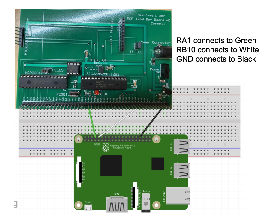
Figure 11. Schematic of UART Connections between PIC32 and Raspberry Pi
Bill of Materials
A bill of materials for this project, which would be required for one starting completely from scratch, is as follows:
| Material | Source | Cost |
|---|---|---|
| Red laser pointer | Amazon | $15.99 |
| Green laser pointer | Amazon | $19.99 |
| Raspberry Pi 3 B | Skovira Lab | $0 |
| USB Webcam | Skovira Lab | $0 |
| Projector | Phillips 101 (or other classroom) | $0 |
| Document Camera | Phillips 101 (or other classroom) | $0 |
References
- Center for Devices and Radiological Health, “Important Information for Laser Pointer Manufacturers,” U.S. Food and Drug Administration, 04-Dec-2017. [Online]. Available: https://www.fda.gov/radiation-emitting-products/laser-products-and-instruments/important-information-laser-pointer-manufacturers#:~:text=This%20means%20that%20pointers%20are,or%20IEC1%20Class%203R. [Accessed: 10-Dec-2021].
- “Laser Classes,” Laser Safety Facts. [Online]. Available: https://www.lasersafetyfacts.com/laserclasses.html. [Accessed: 10-Dec-2021].
- “Does performance differ between Python or C++ coding of opencv?,” NewbeDEV. [Online]. Available: https://newbedev.com/does-performance-differ-between-python-or-c-coding-of-opencv. [Accessed: 12-Dec-2021].
- “Closing,” Morphology, 2003. [Online]. Available: https://homepages.inf.ed.ac.uk/rbf/HIPR2/close.htm. [Accessed: 12-Dec-2021].
- Adrian Rosebrock, “Simple object tracking with OpenCV” PyImageSearch, 2018. [Online]. Available: https://www.pyimagesearch.com/2018/07/23/simple-object-tracking-with-opencv/. [Accessed: 12-Dec-2021].