ECE 4760 Final Project
As a part of the final project for ECE 4760: Digital Systems Design Using Microcontrollers, we worked on a voice controlled version of the Google Dino game on the PIC32 microcontroller. The microcontroller we used is a PIC32MX250F128B microcontroller on the SECABB development board.
We have all been in a situation where we didn’t have access to the internet and to pass time we started playing the Google Dino game. However, the game tends to get a little monotonous with all the key presses and the biggest fear is that if we regain the internet connection, we might lose the progress, especially if we are about to beat a high score. Therefore, for our final project, we wanted to create our own version of the Dino game using the PIC32 microcontroller and the TFT screen which can be controlled with our voice. That way, we could play the game any time we wanted without the fear of losing progress by regaining the internet connection.
The game begins with a start screen with very minimal text saying Press Start!. Once the start button is pressed, the screen updates and the game starts. The game is fairly straightforward with a dino player running. The main task of the game is to keep jumping over obstacles (cactii) and not die. As long as the player is alive, the game keeps on running and generating newer obstacles.
In order to control the dino, the user can use the Jump button which updates the y-velocity of the dino and makes it jump. Once the dino has jumped, the gravity acts on it and its velocity changes each frame. Once the diono hits the ground again, the velocity is reset to 0. Whistling into the microphone can also make the dino jump. Once the dino passes an obstacle, the score is incremented.
If the player fails to make the dino jump and it hits an obstacle, the dino dies and the game over screen is displayed along with the score and high score. In order to start the game again, the user needs to press the Restart button on the GUI.
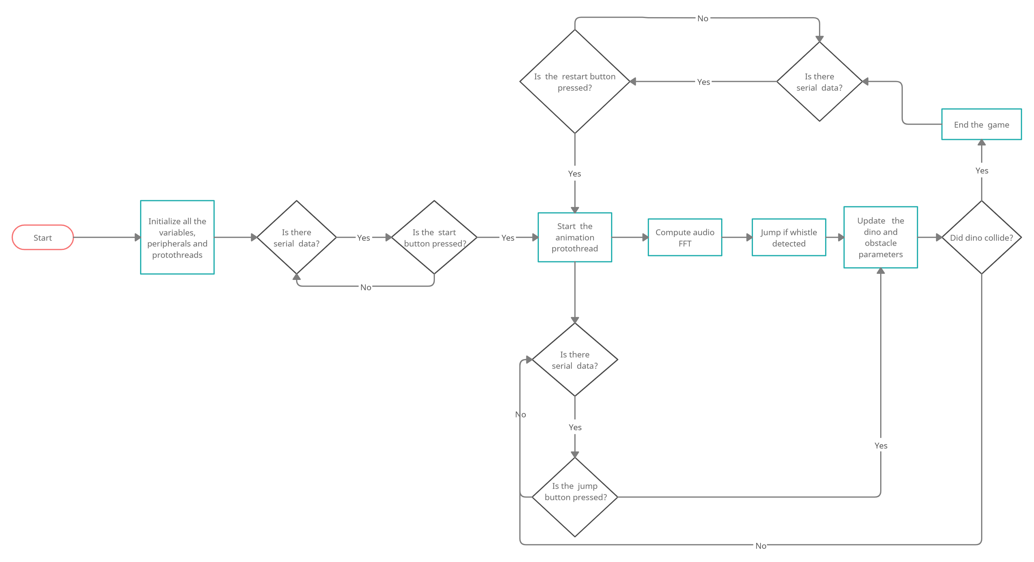
The basic flow diagram of the system is shown below. Note: There is an additional ISR which is not a part of the flow diagram but is a part of the main program.
Sound is a continuous signal. In order to input this continuous signal to the microcontroller, we sample it using the ADC. The rate at which we sample the sound determines the range of frequencies we can recover. The Nyquist–Shannon sampling theorem says that the faster we sample the input signal at, the higher the range of the frequencies we can recover. The basic thing to consider while sampling the signal is: $f_{s} \geq 2 \times f_{highest}$
Where $f_{s}$ is the sampling frequency and $f_{highest}$ is the highest frequency, we need to recover. In our project, we used this relation to calculate the frequency at which the timer should interrupt the flow of the program in order to read the audio input to recover the whistle sound.
Once the audio signal is sampled and broken into N discrete time points, we need to use the Discrete Time Fourier Transform to convert the signal into a discrete number of N frequency signals. The DTFT takes in a real valued argument and an imaginary valued argument. Since we are dealing with sound signals, we only need to concern ourselves with the real valued argument. The discrete-time Fourier transform of a discrete sequence of real or complex numbers x[n], for all integers n, is a Fourier series, which produces a periodic function of a frequency variable. When the frequency variable, ω, has normalized units of radians/sample, the periodicity is 2π, and the Fourier series is:
$X_{2\pi}(\omega) = \sum\limits_{n=-\infty}^{\infty} x[n]e^{-i\omega n}$
In order to compute the DTFT, we use what is called a Fast Fourier Transform. This algorithm allowed us to calculate the DTFT of our sound quite efficiently without using much of our CPU time. A point to remember is that we had to use fixed point arithmetic in order to make our calculations faster as floating-point arithmetic is quite CPU intensive and slow.
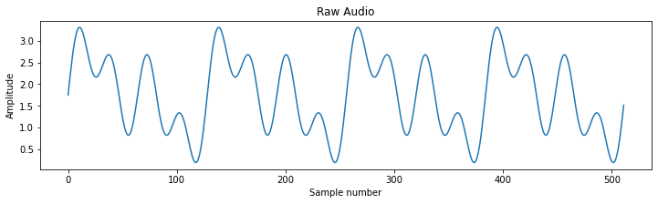
When we compute the FFT of a particular segment of the sound signal, the algorithm assumes that the input to it is a periodic sound signal. In case of a periodic sound signal, the signal would be continuous over the entire time domain. However, our signal is not periodic, and thus, if we apply a fast Fourier transform on it, then we would get sharp high frequency components in our frequency domain. To avoid this, we used a windowing function which would smooth out the signal between different segments. In our case, each segment consisted of 512 samples.
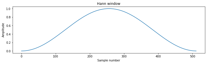
There are various window functions available to choose from. We chose to use the Hann window, which is a cosine-based window function. When we apply a window function, we basically divide the window into the number of samples in our segment, and then multiply every nth sample of the audio signal with the nth sample in the window function. The equation of the Hann window is given below, where N is the total samples in each segment (512 in our case).
$w[n] = [1 - cos(\frac{2\pi n}{N})]$
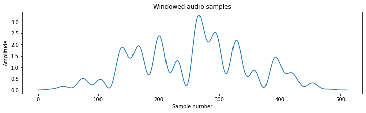
The effect of the window on the audio signal can be seen from the graphs as depicted below.
The output of the FFT algorithm are two arrays (one with real and the other with imaginary values). In order to compute their magnitude, we need to find the root of sum of squares of the respective values. However, as we have established before, the square root is quite a resource intensive operation and takes a long time to compute. In order to find a rough approximation of the magnitude, we use the Alpha Max Beta Min algorithm which says that for two numbers a and b, the root of the sum of their squares is given as: $|z| = max(a, b) + 0.4 \times min(a, b)$
Now, we know that we need to keep our frame rate fixed at 30 fps which is quite hard to achieve as we increase the sample rate and compute the FFT for every 512 samples. We know that the most computationally expensive part of the code is the mathematical computations of the FFT as it is all sorts of addition, multiplication, division etc. of floating-point numbers which takes a really long time to execute. Instead, what we can do to make the computation faster is convert them from floating-point to fixed-point and compute them. The table below shows a comparison of the number of clock cycles it takes to compute the specific operations in fixed and floating-type numbers.
| Cycles / Operation | fix16 | _Accum | float |
|---|---|---|---|
| Add | 5 | 2 | ~60 |
| Multiply | 21 | 28 | ~55 |
| Divide | ~145 | ~145 | ~140 |
| DSP-MAC | 21 | 29 | ~110 |
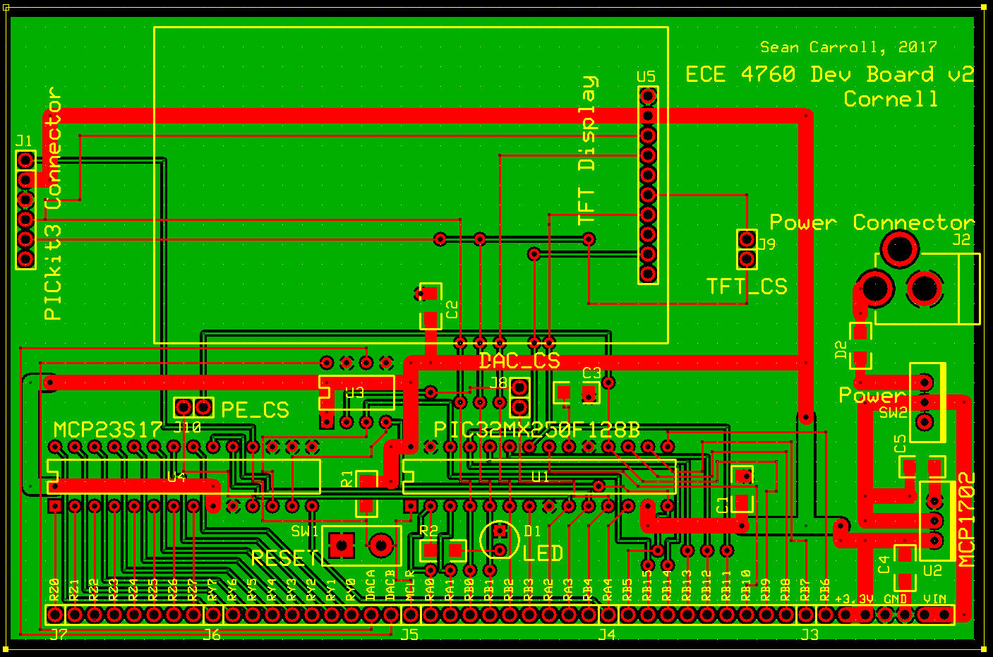
The hardware for the project consists of a PIC32MX250F128B microcontroller setup on a development board (called SECABB). It is connected to the remote desktop via a serial debugger which is used to program the microcontroller and for UART communication between the microcontroller and the GUI.
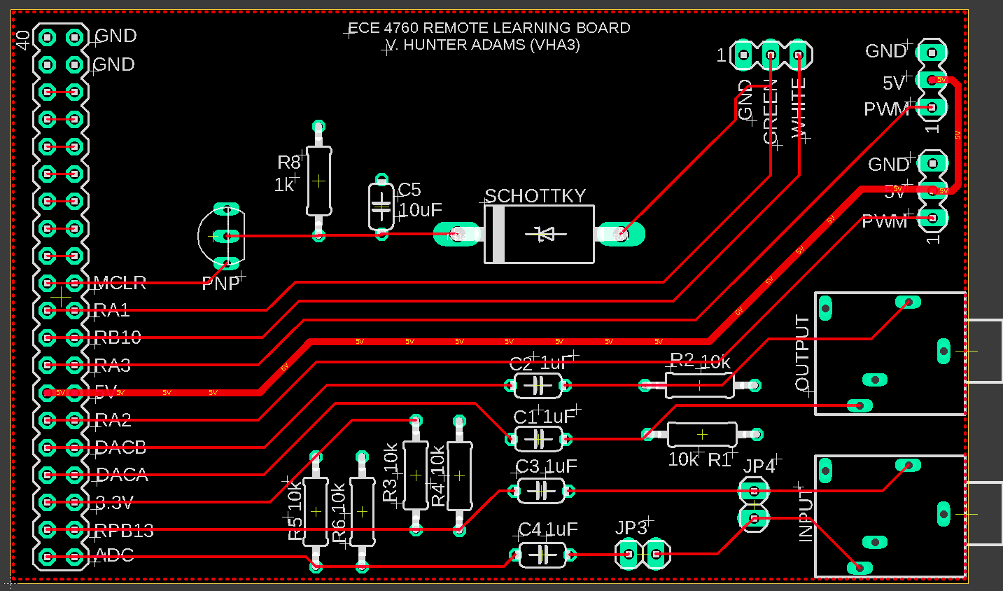
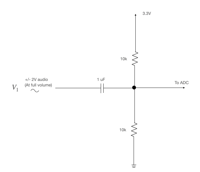
For audio input, we used the built-in analog to digital converter in the PIC32 microcontroller. The ADC has a 10-bit resolution, which means that the 0-3.3V input audio signal amplitude will be resolved into 1024 different values, which means that the microcontroller will read the audio signal with a 3.2mV resolution. The pin we are using to read the ADC input is AN11. The input analog signal is passed onto a sample and hold signal, and at the sampling frequency set, the sample and hold signal converts the analog value to a 10bit digital value and places it in the ADC1BUF0. We then fetch this value from this register and compute FFT once we have 512 values. In our audio sample, there will be a DC noise present. To filter this out, we connected a basic RC high pass filter at the input of the ADC. The filter consists of a 1uF capacitor, and a 10k resistor in the configuration shown in the circuit diagram below. This gives us a cutoff frequency of about 16 Hz. Also, since our input will be -2V to 2V, we also apply a bias at the input of the ADC to shift our signal up by 1.65V.
For audio output, we used a Digital to Analog Converter (DAC) which is communicates with the PIC microcontroller using the SPI communication. The DAC output is also connected to an audio jack which goes back into the remote desktop in order to listen to the generated output. The circuit schematic and the PCB layout can be seen below.
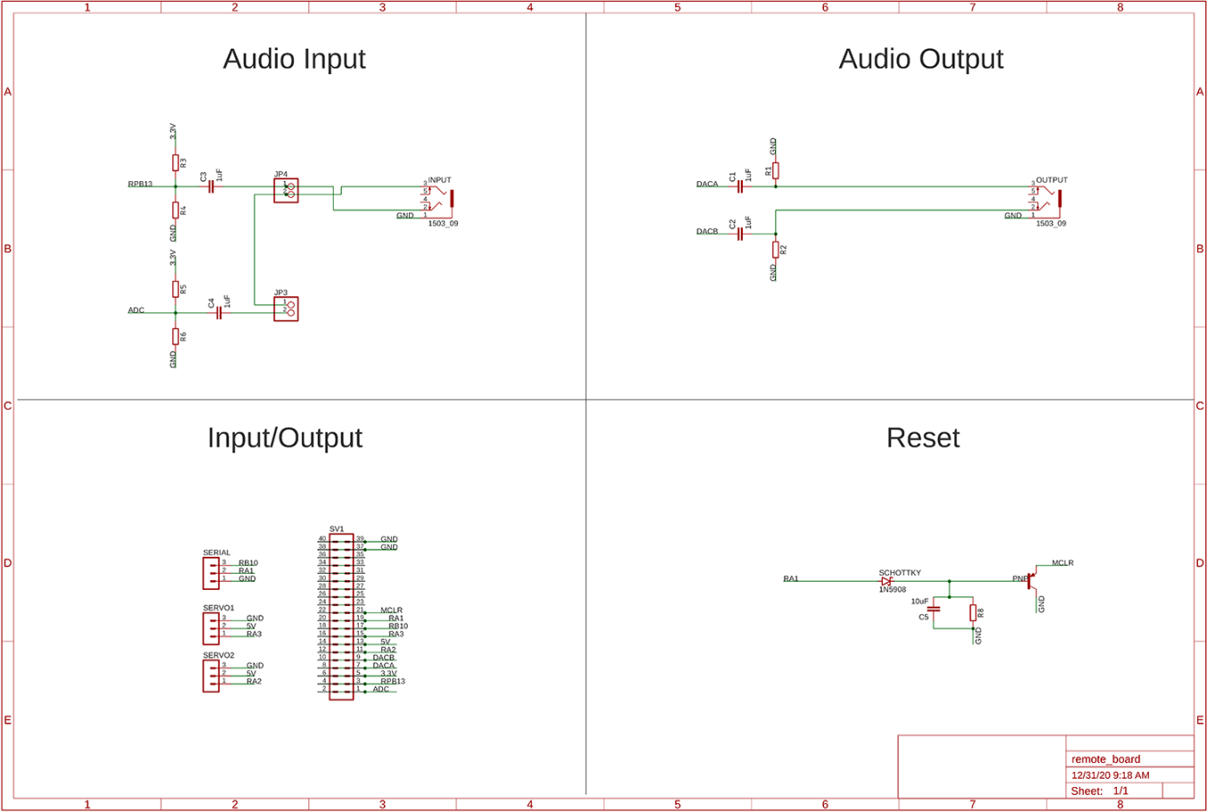
The SECABB has a TFT LCD display attached to it which can be used to display output from the PIC32. The TFT display PCB layout that is used is shown in the images below. The LCD we are using is a 320x240 color LCD with 16-bit color specification. It uses SPI communication from PIC32 to display whatever we want to display using a graphics library ported to PIC32.
Our software design is inspired by the first three labs we performed for the course ECE 4760. The sound generation was inspired from the first lab, the video output was inspired by the second lab and the audio input was inspired by the third lab. Moreover, we also implemented some additional features like DMA and optimized a function in the in-build TFT graphic library.
We feel it is best if we explain the software design in a chronological manner in the form of our weekly reports.
During week 1 of the project, we setup a basic program to display a moving ground frame on the TFT screen attached to the PIC microcontroller. In order to so, we have used the time sharing threading algorithm called protothreads.
In order to create the running ground, we used a simple trick of moving some streaks of white color to the left with each passing frame. Each streak of the ground is a struct stored in an array of grounds. It is implemented as below:
#define GROUND_SIZE 10
struct Ground{
    int x, y, w;
};
struct Ground ground[GROUND_SIZE];
In order to first initialize all the elements of the array, we loop through the array and randomize the x-coordinate, the y-coordinate and the width of the ground. To do so, we use an inline random function as implemented below:
inline int randomRange(int min, int max){
    return (rand() % (max - min)) + min;
}
This random function takes in two arguments: a lower limit and an upper limit. It returns an integer between the said limits. Now that we had the randomRange function, we implemented a for loop to initialize all the parameters in main as below:
for(i = 0; i < GROUND_SIZE; i++){
    ground[i].x = randomRange(0, WIDTH);
    ground[i].y = randomRange(HEIGHT - GROUND_HEIGHT + 10, HEIGHT);
    ground[i].w = randomRange(3, 10);
}
Now that we had an initialized array of streaks on the ground, we needed to update it for every iteration. It was done so by following a simple algorithm:
This algorithm has been implemented as below:
for(i = 0; i < GROUND_SIZE; i++){
    ground[i].x -= SPEED;
    if(ground[i].x + ground[i].w <= 0){
        ground[i].x = WIDTH;
        ground[i].y = randomRange(HEIGHT - GROUND_HEIGHT + 10, HEIGHT);
        ground[i].w = randomRange(3, 10);
    }
}
The output obtained by running the code at the end of week 1 is shown below.
During week 2 of the project, we added some moving obstacles and the dino in the form of some boxes. We then created a Python GUI to interact with the game. The GUI has 3 buttons:
We also used the GUI for debugging purposes.
Once we had our GUI ready, we implemented the jump as well as the collision logic in our code. Once it was up and running, we implemented the voice control feature using ADC input and FFT algorithm.
The code was implemented in various phases as described below.
Just like with implementing the ground, we implemented the obstacles using a struct. However, there is a catch. The ground was implemeted using an array while we only used single variable to implement the obstacle (and reuse it to bring in the next obstacle). We also used a new variable called obsType to keep a track of the type of obstacle (we have 3 different types based on their width and height).
#define OBS_W_0 10
#define OBS_H_0 20
#define OBS_W_1 15
#define OBS_H_1 30
#define OBS_W_2 30
#define OBS_H_2 20

int obsType;

struct Obstacle{
    int x, w, h;
};
struct Obstacle obstacle;
We initialized the obstacle in main as below:
obsType = randomRange(0, 3);
obstacle.x = WIDTH;
if(obsType == 0){
    obstacle.w = OBS_W_0;
    obstacle.h = OBS_H_0;
}
else if(obsType == 1){
    obstacle.w = OBS_W_1;
    obstacle.h = OBS_H_1;
}
else{
    obstacle.w = OBS_W_2;
    obstacle.h = OBS_H_2;
}
Now that we had initialized the obstacle, we needed to update it for every iteration. It was done so by following a simple algorithm:
This algorithm has been implemented as below:
tft_fillRect(obstacle.x, (HEIGHT - GROUND_HEIGHT - ((obstacle.h / 2))), obstacle.w, obstacle.h, ILI9340_BLACK);

obstacle.x -= SPEED;
if(obstacle.x + obstacle.w < 0){
    obsType = randomRange(0, 3);
    obstacle.x = WIDTH + randomRange(0, 50);
    switch(obsType){
        case 0: obstacle.w = OBS_W_0;
                obstacle.h = OBS_H_0;
                break;
        case 1: obstacle.w = OBS_W_1;
                obstacle.h = OBS_H_1;
                break;
        case 2: obstacle.w = OBS_W_2;
                obstacle.h = OBS_H_2;
                break;
    }
}

tft_fillRect(obstacle.x, (HEIGHT - GROUND_HEIGHT - ((obstacle.h / 2))), obstacle.w, obstacle.h, HARD_COLOR);
The output obtained after running this code is given below.
Now that we had implemented the obstacle, we had to implement the Dino. Just like with implementing the obstacke, we implemented the dino using a struct. The dino is a little different from the ground and obstacles. Its x-coordinate is to remain constant and the y-coordinate is to change. It also needs to have a flag in order to keep track of whether the dino is alive or dead and a parameter to keep track of its velocity when it jumps. It is implemented as below.
struct Player{
    int x, y, w, h, vy;
    int alive;
};
struct Player myPlayer;
We initialized the dino (myPlayer) in main as below.
myPlayer.x = 30;
myPlayer.y = 0;
myPlayer.w = 22;
myPlayer.h = 25;
myPlayer.vy = 0;
myPlayer.alive = 1;
Now that we had initialized the dino, we needed to update it for every iteration. It was done so by simply clearing old position of the dino and drawing the new position. The jump logic was implemented later on.
tft_fillRect(myPlayer.x, (HEIGHT - GROUND_HEIGHT - (myPlayer.y + (myPlayer.h / 2))), myPlayer.w, myPlayer.h, ILI9340_BLACK);
tft_fillRect(myPlayer.x, (HEIGHT - GROUND_HEIGHT - (myPlayer.y + (myPlayer.h / 2))), myPlayer.w, myPlayer.h, SOFT_COLOR);
The output obtained after running this code is given below.
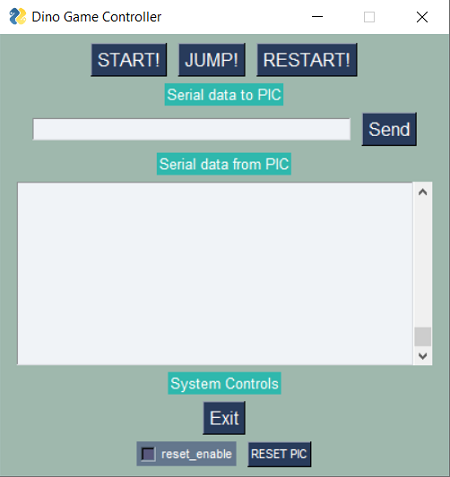
In order to create the GUI, we used the sample code provided by Prof. Bruce Land for the Lab 0 of ECE 4760 course and modified it in order to create our GUI. In particular, we changed the layout list to add 3 buttons to be used. We also had to bind the corrosponding ButtonRelease functionality.
layout = [[sg.RealtimeButton('START!', key = 'pushbut01', font = 'Helvetica 12'),
           sg.RealtimeButton('JUMP!', key = 'pushbut02', font = 'Helvetica 12'),
           sg.RealtimeButton('RESTART!', key = 'pushbut03', font = 'Helvetica 12')],

          [sg.Text('Serial data to PIC', background_color = heading_color)],
          [sg.InputText('', size = (40, 10), key = 'pic_input', do_not_clear = False, enable_events = False, focus = True),
           sg.Button('Send', key = 'pic_send', font = 'Helvetica 12')],

          [sg.Text('Serial data from PIC', background_color = heading_color)],
          [sg.Multiline('', size = (50, 10), key = 'console', autoscroll = True, enable_events = False)],

          [sg.Text('System Controls', background_color = heading_color)],
          [sg.Button('Exit', font = 'Helvetica 12')],
          [sg.Checkbox('reset_enable', key = 'r_en', font = 'Helvetica 8', enable_events = True),
           sg.Button('RESET PIC', key = 'rtg', font = 'Helvetica 8')
         ]]

window['pushbut01'].bind('<ButtonRelease-1>', 'r')
window['pushbut02'].bind('<ButtonRelease-1>', 'r')
window['pushbut03'].bind('<ButtonRelease-1>', 'r')
The generated GUI looks as shown below.
Now that we had created the GUI, we started working on the implementing the jump algorithm. In order to do so, we defined the gravity and the initial velocity at which it jumped. Then for every iteration, we changed the velocity based on gravity and changed the y-coordinate based on the velocity.
In order implement the jump algorithm, we added a new protothread to serially communicate with the Python GUI. When we press the jump button, we simply change the dino velocity to a predefined velocity and increment the y-coordinate by 1. It has been implemented as below.
Note: We also implemented the Start functionality to prevent the game from starting before the user is ready to play. It was quite simple to do, using the startGame flag.
#define GRAVITY 1.2
#define JUM_VEL 15

char startGame = 0;
char newButton = 0;
char buttonID, buttonValue;
We initialized the start screen to display Press Start in the main as below.
tft_setTextSize(4);
tft_setTextColor(SOFT_COLOR);
tft_setCursor(25, 100);
tft_writeString("Press Start!");
The start screen looks as shown below.
Now that we had our start screen ready, we added a protothread to detect for start button press and start the game if the button is pressed. It was implemented as shown below.
if(buttonID == 1 && buttonValue == 1 && startGame == 0){
    startGame = 1;
    tft_fillRect(0, 0, WIDTH, HEIGHT, ILI9340_BLACK);
}
Now once the game had started, we wanted to check for the jump button press. It was implemented in the same protothread as follows.
if(buttonID == 2 && buttonValue == 1 && myPlayer.y == 0 && startGame){
    myPlayer.vy = JUM_VEL;
    myPlayer.y += 1;
}
Now, once we had updated the velocity and the y-coordinate of the dino, it was fairly straightforward to update the dino and make it jump up and back down. We implemented the logic in the animation thread as below.
if(myPlayer.y > 0){
    myPlayer.y += myPlayer.vy;
    myPlayer.vy -= GRAVITY;
}
else if(myPlayer.y < 0){
    myPlayer.y = 0;
    myPlayer.vy = 0;
}
After implementing the jump algorithm, we tested the code out using the GUI. The result is shown below.
Now that everything was ready, we only needed to implement the collision algorithm to finish the game. To do so, we used a simple algorithm to keep a track of hitboxes and test if the hitboxes collide. Once we detect that hitboxes have collided, we simply set the alive flag to false and display the death message. It is implemented as below.
if((myPlayer.x + myPlayer.w > obstacle.x) && (myPlayer.x < obstacle.x + obstacle.w) && (myPlayer.y < obstacle.h)){
    myPlayer.alive = 0;
    tft_setTextSize(4);
    tft_setTextColor(SOFT_COLOR);
    tft_setCursor(5, 60);
    tft_writeString("!!!!!DEAD!!!!!");
}
After implementing the collision algorithm, we tested the code out using the GUI. The result is shown below.
Now that our basic game was almost ready, the only thing that was left to do was add a restart functionality after our player died. It was implemented as below.
if(buttonID == 3 && buttonValue == 1){
    startGame = 0;
    tft_fillRect(0, 0, WIDTH, HEIGHT, ILI9340_BLACK);
    tft_setTextSize(4);
    tft_setTextColor(SOFT_COLOR);
    tft_setCursor(25, 100);
    tft_writeString("Press Start!");

    obsType = randomRange(0, 3);
    obstacle.x = WIDTH;
    if(obsType == 0){
        obstacle.w = OBS_W_0;
        obstacle.h = OBS_H_0;
    }
    else if(obsType == 1){
        obstacle.w = OBS_W_1;
        obstacle.h = OBS_H_1;
    }
    else{
        obstacle.w = OBS_W_2;
        obstacle.h = OBS_H_2;
    }

    myPlayer.y = 0;
    myPlayer.vy = 0;
    myPlayer.alive = 1;
}
At this stage our game was completely ready (except for the graphics using bitmaps). Therefore, we moved on to the next stage which was implementation of the voice control feature.
This was probably the most challenging part of the entire project. In order to get the voice input, we used the Analog to Digital Converter (ADC). The ADC was triggered by a timer interrupt. Once we got the ADC input in an array, we fed the array to a Fast Fourier Transform (FFT) function. The FFT function computes the FFT of the input and provides a range of frequency bins. We then computed which bin has the highest power and then used the bin to compute the frequency range with most power. In order to use the ADC, we used the following parameters. Here F is the clock frequency and Fs is the sampling frequency.
#define F 40000000
#define Fs 4000

#define PARAM1 ADC_FORMAT_INTG16 | ADC_CLK_AUTO | ADC_AUTO_SAMPLING_OFF
#define PARAM2 ADC_VREF_AVDD_AVSS | ADC_OFFSET_CAL_DISABLE | ADC_SCAN_OFF | ADC_SAMPLES_PER_INT_1 | ADC_ALT_BUF_OFF | ADC_ALT_INPUT_OFF
#define PARAM3 ADC_CONV_CLK_PB | ADC_SAMPLE_TIME_5 | ADC_CONV_CLK_Tcy2
#define PARAM4 ENABLE_AN11_ANA
#define PARAM5 SKIP_SCAN_ALL
We setup Timer 2 to interrupt at 4000 Hz as below.
OpenTimer2(T2_ON | T2_SOURCE_INT | T2_PS_1_1, F / Fs);
ConfigIntTimer2(T2_INT_ON | T2_INT_PRIOR_2);
mT2ClearIntFlag();
Next, we configured the ADC to read the input as below.
CloseADC10();
SetChanADC10(ADC_CH0_NEG_SAMPLEA_NVREF | ADC_CH0_POS_SAMPLEA_AN11);
OpenADC10(PARAM1, PARAM2, PARAM3, PARAM4, PARAM5);
EnableADC10();
In order to read the ADC input, we used a counter variable, an input variable and a fixed point array to store the most recent 512 input values.
#define nSamp 512
#define nPixels 256
#define N_WAVE 512
#define LOG2_N_WAVE 9

_Accum v_in[nSamp];

volatile int adc_9 = 0;
int counter = 0;

void __ISR(_TIMER_2_VECTOR, ipl2) Timer2Handler(void){
    mT2ClearIntFlag();
    adc_9 = ReadADC10(0);
    AcquireADC10();

    v_in[counter] = int2Accum(adc_9);
    counter++;
    if(counter == 512){
        counter = 0;
    }
}
In order to compute the FFT of the input signal, we used an FFT function which takes in a real array and an imaginary array as an input and returns the output in the same real and imaginary arrays. In our case, our input will completely be stored in the real array as it is a voice signal input and the imaginary array will be all 0s.
void FFTfix(_Accum fr[], _Accum fi[], int m){
    int mr, nn, i, j, L, k, istep, n;
    _Accum qr, qi, tr, ti, wr, wi;

    mr = 0;
    n = 1 << m;
    nn = n - 1;
    for(m = 1; m <= nn; ++m){
        L = n;
        do{
            L >>= 1;
        }
        while(mr + L > nn);
        mr = (mr & (L - 1)) + L;
        if(mr <= m){
            continue;
        }
        tr = fr[m];
        fr[m] = fr[mr];
        fr[mr] = tr;
    }

    L = 1;
    k = LOG2_N_WAVE - 1;
    while(L < n){
        istep = L << 1;
        for(m = 0; m < L; ++m){
            j = m << k;
            wr =  Sinewave[j + N_WAVE / 4];
            wi = -Sinewave[j];
            for(i = m; i < n; i += istep){
                j = i + L;
                tr = (wr * fr[j]) - (wi * fi[j]);
                ti = (wr * fi[j]) + (wi * fr[j]);
                qr = fr[i] >> 1;
                qi = fi[i] >> 1;
                fr[j] = qr - tr;
                fi[j] = qi - ti;
                fr[i] = qr + tr;
                fi[i] = qi + ti;
            }
        }
        --k;
        L = istep;
    }
}
We also needed to define a fixed point sine table to be used by the FFT function and initialize it in main.
_Accum Sinewave[N_WAVE];

for (i = 0; i < N_WAVE; i++){
    Sinewave[i] = float2Accum(sin(6.283 * ((float) i) / N_WAVE) * 0.5);
}
For the final part of the voice control implementation, we implemented the FFT function to our voice input in the animation protothread following a simple algorithm:
fr.fi as all 0s.FFTFix to compute Fast Fourier Trasnform and store the result in fr and fi.Alpha Max Beta Min algorithm and store it in fr.This Hann window was implemented as below.
_Accum window[N_WAVE];

for (i = 0; i < N_WAVE; i++){
    window[i] = float2Accum(1.0 - cos(6.283 * ((float) i) / (N_WAVE - 1)));
}
The voice detection algorithm was implemented as below.
#define FREQ_UPPER 1800
#define FREQ_LOWER 1500

_Accum maxFreq;

for(sample_number = 0; sample_number < nSamp - 1; sample_number++){
    fr[sample_number] = v_in[sample_number] * window[sample_number];
    fi[sample_number] = 0 ;
}
FFTfix(fr, fi, LOG2_N_WAVE);

for(sample_number = 0; sample_number < nPixels; sample_number++){
    fr[sample_number] = abs(fr[sample_number]);
    fi[sample_number] = abs(fi[sample_number]);
    fr[sample_number] = max(fr[sample_number], fi[sample_number]) + (min(fr[sample_number], fi[sample_number]) * zero_point_4);
}
static maxPower = 3;
for(sample_number = 3; sample_number <= nPixels; sample_number++){
    if(fr[sample_number] > fr[maxPower]){
        maxPower = sample_number;
    }
}

maxFreq = ((int2Accum(Fs) / int2Accum(512)) * int2Accum(maxPower));
printf("Max Power: %d\n", Accum2int(maxFreq));
if(maxFreq < int2Accum(FREQ_UPPER) && maxFreq > int2Accum(FREQ_LOWER) && myPlayer.y == 0){
    myPlayer.vy = JUM_VEL;
    myPlayer.y += 1;
}
Note: We start computing the maximum frequency from the $3^{rd}$ bin as there is a DC offset which will always have the maximum power.
A video demonstration at the end of week 2 is attached below.
During week 3 of the project, we worked on replacing the dino and obstacle blocks with bitmap images of a cartoon dinosaur and 3 different types of cactii to make it aesthetically pleasing. In order to do so, we first used the predefined tft_drawBitmap() function and successfully implemented the dino and cactii graphics in the game. However, we realized that the function is not optimized and takes a lot of CPU cycles to run. Thus, we digged into the header files and created our own optimized function for drawing bitmaps.
Next, we implemented the live score and high score functionality in the game.
In order to implement the graphics for the dino and cactii, we downloaded stock images of 3 different cactii, and 3 configurations of the dino - jump position, running position 1 and running position 2.
In order from left to right: small cactus, large cactus and multiple cactii.


In order from left to right: dino jump, running position 1 and running position 2.


In order to display these images in the game, we needed to convert them in a form which a microcontroller could understand. This form is known as a bitmap. A bitmap is basically an array of pixels where each bit of the array signifies whether a pixel is dark or light. If the pixel is light, the bit is set to 1 and if the pixel is dark, the bit is set to 0. In order to conserve space, the pixels are represented in a hexdecimal format so that each element of the array represents a series of 8 pixels.
In order to convert these PNG images in the bitmap format, we used LCD Image Converter. We followed the following steps for this conversion:
Options > Conversion.Monochrome and click Show Preview.The above conversion was repeated for all six images and we stored the resultant arrays in a file called BitMap.h. Every single array is of the type const unsigned char. We used const because the bitmap will remain constant throught the execution of the program and will be stored in the flash memory.
The provided tft_gfx.h library has a predefined function called tft_drawBitmap() which takes in the following parameters to draw the image:
We implemented the code as below.
We first included the bitmap library.
#include "BitMap.h"
We then defined RUNNER_FRAMES constant value and a variable runner which help us in creating an illusion of the dino running.
#define RUNNER_FRAMES 10
char runner = 0;
The next step was to replace all the tft_fillRect() functions in the animation protothread with the tft_drawBitmap() function to implement the dino cactii graphics.
Note: To implement the cactii graphics, we had to use a switch case which draws the correct bitmap for the cactii based on the variable obsType.
switch(obsType){
    case 0: tft_drawBitmap(obstacle.x, (HEIGHT - GROUND_HEIGHT - ((obstacle.h / 2))), obsTypeZer, obstacle.w, obstacle.h, ILI9340_BLACK);
            break;
    case 1: tft_drawBitmap(obstacle.x, (HEIGHT - GROUND_HEIGHT - ((obstacle.h / 2))), obsTypeOne, obstacle.w, obstacle.h, ILI9340_BLACK);
            break;
    case 2: tft_drawBitmap(obstacle.x, (HEIGHT - GROUND_HEIGHT - ((obstacle.h / 2))), obsTypeTwo, obstacle.w, obstacle.h, ILI9340_BLACK);
            break;
}

//After updating the obstacle parameters

switch(obsType){
    case 0: tft_drawBitmap(obstacle.x, (HEIGHT - GROUND_HEIGHT - ((obstacle.h / 2))), obsTypeZer, obstacle.w, obstacle.h, HARD_COLOR);
            break;
    case 1: tft_drawBitmap(obstacle.x, (HEIGHT - GROUND_HEIGHT - ((obstacle.h / 2))), obsTypeOne, obstacle.w, obstacle.h, HARD_COLOR);
            break;
    case 2: tft_drawBitmap(obstacle.x, (HEIGHT - GROUND_HEIGHT - ((obstacle.h / 2))), obsTypeTwo, obstacle.w, obstacle.h, HARD_COLOR);
            break;
}
After updating the player parameters, we had to draw the appropriate dino image. We used the following three conditions to draw the dino:
runner variable is between 0 and RUNNER_FRAMES / 2, then draw the dino running position 1 bitmap.runner variable is between RUNNER_FRAMES / 2 and RUNNER_FRAMES, then draw the dino running position 2 bitmap.Once the runner variable hits RUNNER_FRAMES, it will reset to 0.
if(myPlayer.y > 0){
    tft_drawBitmap(myPlayer.x, (HEIGHT - GROUND_HEIGHT - (myPlayer.y + (myPlayer.h / 2))), dinoJumpUp, myPlayer.w, myPlayer.h, SOFT_COLOR);
}
else{
    if(runner > RUNNER_FRAMES / 2){
        tft_drawBitmap(myPlayer.x, (HEIGHT - GROUND_HEIGHT - (myPlayer.y + (myPlayer.h / 2))), dinoRunOne, myPlayer.w, myPlayer.h, SOFT_COLOR);
    }
    else{
        tft_drawBitmap(myPlayer.x, (HEIGHT - GROUND_HEIGHT - (myPlayer.y + (myPlayer.h / 2))), dinoRunTwo, myPlayer.w, myPlayer.h, SOFT_COLOR);
    }
}
runner = (runner + 1) % RUNNER_FRAMES;
After implementing the bitmaps, we tested the code out using the GUI. The result is shown below.
As we can see from the result, the amount of extra time we were left with is 1 millisecond for a specific frame with the multi cactus image. This is not a lot considering that it was about 7-8 milliseconds before implementing the graphics. Therefore, there was a pressing need to optimize the process of drawing bitmap.
In order to optimize the function, we dug into the library and studied how each function is implemented. Particularly, the tft_drawBitmap() function is implemented in the following manner:
byteWidth and counter variables i & j.tft_drawPixel() function.At first glance, this doesn't look particularly unoptimized. However, digging in deeper, we found that calling the tft_drawPixel() function for all the pixels is pretty time consuming as the tft_drawPixel() function is implemented as follows:
This row and column address configuration for all the pixels is quite time consuming and redundant. On the other hand, comparing it to the tft_fillRect() function, this function is implemented as follows:
This function is extremely optimized as we need to set the address window only once. Therefore, we combined the two functions to create a new function called drawBitmap() which takes in the same set of arguments as the tft_drawBitmap() function (and is therefore interchangeable). It was implemented as follows:
tft_spiwrite16() function.0xFFFF directly to the TFT using the tft_spiwrite16() function to draw a black background.Note: This function assumes that the background is black in color. It can be optimized to take a different background color.
The implemented function is shown below.
#define pgm_read_byte(addr) (*(const unsigned char *)(addr))
void drawBitmap(short x, short y, const unsigned char *bitmap, short w, short h, unsigned short color){
    if((x >= _width) || (y >= _height)) return;
    if((x + w - 1) >= _width)  w = _width  - x;
    if((y + h - 1) >= _height) h = _height - y;

    tft_setAddrWindow(x, y, x + w - 1, y + h - 1);
    _dc_high();
    _cs_low();

    short i, j, byteWidth = (w + 7) / 8;
    for(j = 0; j < h; j++){
        for(i = 0; i < w; i++){
            if(pgm_read_byte(bitmap + j * byteWidth + i / 8) & (128 >> (i & 7))) {
                tft_spiwrite16(color);
            }
            else{
                tft_spiwrite16(0x0000);
            }
        }
    }

  _cs_high();
}
After implementing the bitmaps using our optimized function, we tested the code out again using the GUI. The result is shown below.
As we can see from the result, the amount of extra time we were left with is 7 milliseconds for a specific frame with the multi cactus image. This is a huge improvement as compared to the unoptimized version of the code. This timing difference is even greated for larger bitmaps as there are more pixels to draw.
At this point our game was almost ready. One small thing that was left was keeping a track of score and high score. In order to do so, we initialized two variables: score and highScore.
int score = 0, highScore = 0;
In order to keep a track of the score, we increment the score as soon as the obstacle has passed the frame in the animation protothread. Next, we compare if the current score is greater than the high score. If it is, we change the high score.
if(obstacle.x + obstacle.w < 0){
    score++;
    if(score > highScore){
        highScore = score;
    }
}
Moreover, we needed to add the score reset feature in the reset button functionality. Therefore, we modified the reset button condition in the button protothread by adding the following statement to it.
score = 0;
At this point the score and high score were implemented. All that was left to do was print them out on the screen. In order to do so, we #defineed a few parameters which kept a track of the screen coordinates as to where to show the score.
#define SCORE_X_OFFSET1 5
#define SCORE_X_OFFSET2 150
#define SCORE_Y_OFFSET1 5
#define SCORE_Y_OFFSET2 30
Next, we implemented the following lines of code in the start button condition in the button protothread in order to print out the score as soon as the game starts. The tft_setTextSize() is used to set the size of the text to be printed. tft_setTextColor() is used to change the color of the text to be printed. The tft_setCursor() function takes in two arguments: the x-coordinate and the y-coordinate of the top left corner of the text. In order to print a string on the screen, we used the tft_writeString(). Lastly, in order to print some variables on the screen, we had to use the sprintf() function to first store the variable in a char array and then send the char array to the screen in order to print it.
tft_setTextSize(2);
tft_setTextColor(SOFT_COLOR);
tft_setCursor(SCORE_X_OFFSET1, SCORE_Y_OFFSET1);
tft_writeString("Your Score:");
tft_setCursor(SCORE_X_OFFSET1, SCORE_Y_OFFSET2);
tft_writeString("High Score:");
tft_setCursor(SCORE_X_OFFSET2, SCORE_Y_OFFSET1);
sprintf(buffer, "%2d", score);
tft_writeString(buffer);
tft_setCursor(SCORE_X_OFFSET2, SCORE_Y_OFFSET2);
sprintf(buffer, "%2d", highScore);
tft_writeString(buffer);
Next, everytime the score changes (when the obstacle moves out of the frame), we changed the text printed on the screen. We implemented it by adding the following lines in the animation protothread. We first erase the previous value of the score and highscore by printing them in black and then print the updated values using the desired color.
if(obstacle.x + obstacle.w < 0){
    tft_setTextColor(ILI9340_BLACK);
    tft_setCursor(SCORE_X_OFFSET2, SCORE_Y_OFFSET1);
    sprintf(buffer, "%2d", score);
    tft_writeString(buffer);
    tft_setCursor(SCORE_X_OFFSET2, SCORE_Y_OFFSET2);
    sprintf(buffer, "%2d", highScore);
    tft_writeString(buffer);

    //Update the score and high score

    tft_setTextColor(SOFT_COLOR);
    tft_setCursor(SCORE_X_OFFSET2, SCORE_Y_OFFSET1);
    sprintf(buffer, "%2d", score);
    tft_writeString(buffer);
    tft_setCursor(SCORE_X_OFFSET2, SCORE_Y_OFFSET2);
    sprintf(buffer, "%2d", highScore);
    tft_writeString(buffer);
}
A video demonstration at the end of week 3 is attached below.
During week 4 of the project, we worked on adding the sound effects. In order to do so, we first used MATLAB to convert some wav audio files into a large array and then used that array to send data directly to the DAC using DMA.
Next, we tweaked the background color a bit to make the display more presentable.
In order to add the audio in game, we first had to covert it into a form which can directly be read by the microcontroller. Moreover, it had to be in a format that can be directly pushed to the DAC. Hence, we also had to append the 4 DAC configuration bits in the MSB of each element of the audio array.
First, we defined the upper and lower bounds of the audio file in terms of the audio sample number. This was done to remove any unwanted sections of the audio. Next, we defined the FILE_NAME and the TEXT_FILE. These are the audio input file name and the output text file name respectively. Lastly, we defined the BitRate which is the new sampling frequency of the audio. This was done to reduce the size of the audio array. Note: Reducing the bitrate of the audio also reduces the audio quality.
UPPER_RANGE = %Your Upper Range%
LOWER_RANGE = %Your Upper Range%
FILE_NAME = %Audio File Name%
TEXT_FILE = %Text File Name%
BitRate = 8000
Range = [LOWER_RANGE, UPPER_RANGE];
Next we used the audioread() function to read the audio file into an array y and get its default sampling frequency Fs. In order to change the sampling frequency, we used the resample() function to change its bitrate. Note: This function requires the DSP toolbox to be installed in MATLAB to work properly. The audio file we read was a 2 channel audio, hence we sliced it down to a single channel and stored it in ys as a column matrix. The amplitude of the audio input stored in ys ranges from -1 to 1. However, we have a 12-bit DAC. Therefore, we had to rescale the amplitude from 0 to 4095. This was done using the rescale() function. Laslty, we force casted each element of the audio to a uint16 data type in order to make it compatible with the DAC.
[y, Fs] = audioread(FILE_NAME, Range);
yn = resample(y, BitRate, Fs);
ys = yn(:, 1);
yqfinal = rescale(ys, 0, 4095);
ysfinal = cast(yqfinal, 'uint16');
We then opened the text file in write mode using the fopen() function. Then we used a for loop to traverse through every element of the audio array and append the DAC configuration bits to it by performing a bitwise OR operation using the bitor() function. The elements are then written into the text file using the fprintf() function. After all elements are written in the text file, we closed the file using the fclose() function.
file = fopen(TEXT_FILE, 'w');
for i = 1 : length(ysfinal)
    yfinal(i) = bitor(ysfinal(i), 0b0011000000000000);
    fprintf(file, "%d, ", yfinal(i));
end
fclose(file);
The above conversion was repeated for all audio files and we stored the resultant arrays in a file called Audio.h. Every single array is of the type const unsigned short. We used const because the audio will remain constant throught the execution of the program and will be stored in the flash memory.
In order to implement the audio functionality, we used Direct Memory Access (DMA). We chose DMA because it is a hardware peripheral functionality and as a result doesn't use up any clock cycles to run. Moreover, once setup, it can be triggered from any point in the code. We implemented the code as below.
We first included the audio library.
#include "Audio.h"
We the defined a few parameters. These are namely the number of bytes in the audio arrays (twice the number of elements in the arrays since it is a short data type) and the DMA channels (we are using channels 2 and 3 as channels 0 and 1 are used by the serial protothread). We also defined a SPI_CLK_DIV as the maximum SPI frequency is 20MHz.
#define JUMP_AUDIO_SIZE 23156
#define DEAD_AUDIO_SIZE 35670
#define DMA_CHANNEL2 2
#define DMA_CHANNEL3 3
#define SPI_CLK_DIV 2
In order to use the DMA, we need to configure a timer which overflows and throws an interrupt at the same rate as the bitrate of the audio. This is to ensure that the audio is played at the correct frequency. In order to do so, we used the Timer 3 in PIC32 and configured it to throw an interrupt after every 5000 CPU cycles (since our bitrate is 8kHz and the CPU frequency is 40MHz).
OpenTimer3(T3_ON | T3_SOURCE_INT | T3_PS_1_1, 5000);
Next, we configured the SPI channel 2 to communicate with the DAC. To do so, we enabled the SPI in 16-bit mode and in the master configuration. We also used SPICON_FRMEN and SPICON_FRMPOL flags to ensure that the SPI is configured in the framed SPI mode as we cannot toggle the chip select line in software while using DMA. Next, we mapped the SPI data out pin to RPB5 and the SPI chip select line to RPA3 pin on the board.
SpiChnOpen(SPI_CHANNEL2, SPI_OPEN_ON | SPI_OPEN_MODE16 | SPI_OPEN_MSTEN | SPI_OPEN_CKE_REV | SPICON_FRMEN | SPICON_FRMPOL, SPI_CLK_DIV);
PPSOutput(2, RPB5, SDO2);
PPSOutput(4, RPA3, SS2);
In order to open the DMA channel, we used the DmaChnOpen() command. We used the higher priority for deadAudio as that takes priority over jumps. Moreover, we used the DMA_OPEN_DEFAULT flag as we want our audio samples to play only once and then stop. Next, in order to configure the transfers, we used the DmaChnSetTxfer() function to set the transfer parameters. It takes in the arguments as the dma channel, the source address, the destination address, the source size, the destination size and the transferred cell size in the given order. Lastly, we setup the DMA event control to timer 3 IRQ as it will control the DMA transfers once the DMA channel has been enabled.
DmaChnOpen(DMA_CHANNEL2, 3, DMA_OPEN_DEFAULT);
DmaChnSetTxfer(DMA_CHANNEL2, jumpAudio, (void*)&SPI2BUF, JUMP_AUDIO_SIZE, 2, 2);
DmaChnSetEventControl(DMA_CHANNEL2, DMA_EV_START_IRQ(_TIMER_3_IRQ));

DmaChnOpen(DMA_CHANNEL3, 0, DMA_OPEN_DEFAULT);
DmaChnSetTxfer(DMA_CHANNEL3, deadAudio, (void*)&SPI2BUF, DEAD_AUDIO_SIZE, 2, 2);
DmaChnSetEventControl(DMA_CHANNEL3, DMA_EV_START_IRQ(_TIMER_3_IRQ));
In order to play the audio, we used the DmaChnEnable() function to start DMA transfers to the DAC. This function is called whenever the dino jumps to play the jump audio or the dino dies to play the death audio.
A video demonstration at the end of week 4 is attached below.
We wanted our game to run at 30 fps as it looks most aesthetically pleasing to the eyes. Therefore, each computation cycle (and hence frame) must be executed within 33ms. To keep a track of whether we are meeting this timing deadline, we printed out the time remaining in each computation cycle, after all the computations were done. If this number was a positive number, then that implies that we are able to meet the deadline. After numerous cycles of testing, we conclude that our game is running at 30 fps and the time metric doesn't go below 0 for any frame.
In order to test the optimization provided by our drawBitmap() function, we compared the amount of time left after updation of each frame in order to maintain a constant frame rate of 30 fps. We found out that for a frame with the largest group of cactii, there is about 1 millisecond left in case of the unoptimized tft_drawBitmap() function.
However, for the same frame with the largest group of cactii, there is about 7 milliseconds left in case of the optimized drawBitmap() function.
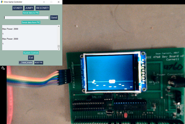
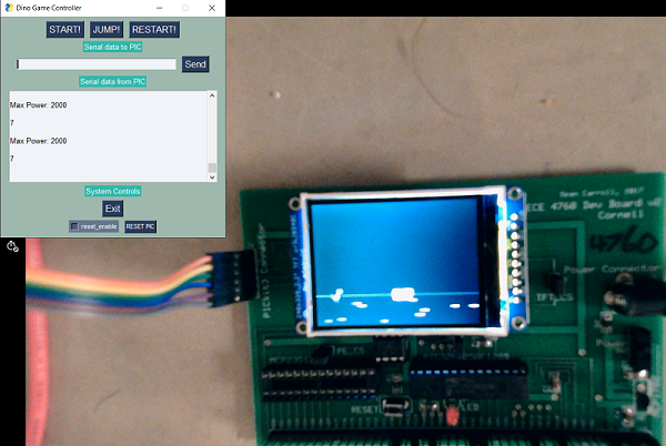
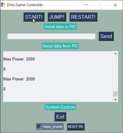
One crucial aspect of the game being controlled using whistle was that it must respond to the frequencies of the whistle only and not the frequencies of any other noises- talking, background hum, etc. To test that the game responds only to frequencies in a given range (1500Hz to 1800Hz), we played the game using a tone generator. The range of frequencies to which the dino jumped are given below:
These values are within 3Hz of the given range, which makes sense because the size of each bracket in the FFT is 4Hz (512 point FFT in a 2kHz range). Thus, we were successful in getting the dino to respond only to whistle frequencies.
Our final dino game works exactly as we expected it to and follows everything we outlined in the final project proposal. We met all the goals we outlined and the game behaved exactly as we expected it to in the demo. If we were to do this project again, we would add additional flash memory to make the game more complex. We would like to add extra sounds, maybe even birds for the dino to duck under.
We believe there is no intellectual property associated with this project. We have merely replicated an open-source game using our own code and linked all the associated softwares appropriately.
This project does not jeopardise the safety of the users or endangers the environment, and we believe our project does not have confilict of interest with any party. In accordance with the IEEE Code of Ethics, we actively seeked help and suggestions from our professors and TAs on the project and asked for ideas for how to make it better.
There are no legal considerations relevant to this project.
The following are the commented code listings used throughout the project:
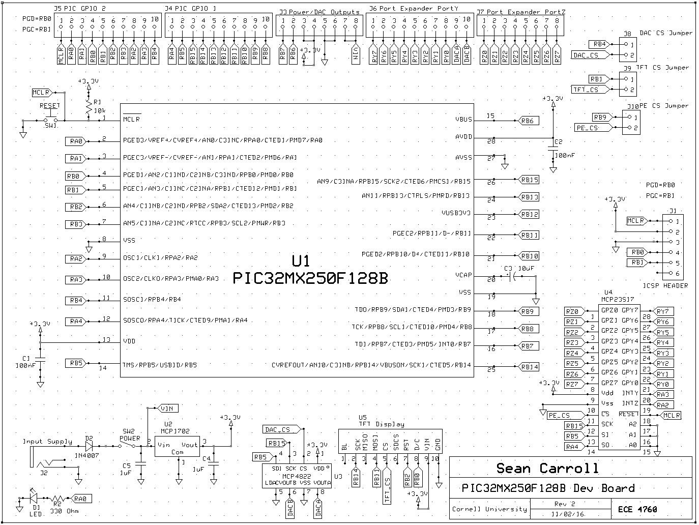
The schematics of the SECABB is as shown below.
Our project did not require any additional purchases than what we were already provided with for the lab work of the course. The cost of these components is as follows:
Total: \$34.30
We both live in the same apartment, so we were able to work together in person and contribute equally to all sections of the project. Instead of splitting the project into tasks for each of us to work on separately, we chose to brainstorm and code the project together.