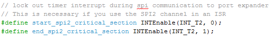
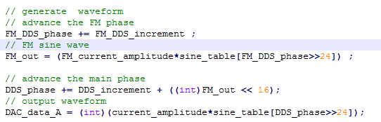
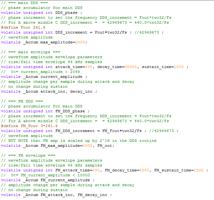
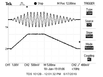
The basic building block for enther additive synthesis or FM synthesis is a sine wave burst with controllable attack, sustain, and decay rates. This example uses the GCC stdfix variable type _Accum to implement s16.15, 2's complement, fixed point. Fixed point is considerably faster than floating point on this architecture. The DDS synthesis is performed in an ISR running at 44KHz, so with only 909 cpu cycles (at 40 MHz cpu clock) between samples efficiency is important. The image below shows an audio burst on the top trace of a 440 Hz sine wave modulated by the amplitude envelope shown in the bottom trace. Rise time (attack time) is 500 synthesis sample times, sustain is 500 sample times, and decay time is 1000 sample times. The example code also handles a keypad connected by port expander which shares an SPI channel with the audio DAC. The sharing requires that a thread and the ISR share the SPI channel, so the thread has to be able to lock out the ISR using a critical section. Also, the ISR has to wait for any executing SPI transaction to end. This code runs on the SECABB board using the Protothreads 1_3_2 environment described on the development board page. The variable declarations for a full FM synthesis give parameter values for string-like and rod-like (wav) sounds. The attached code shows six possible FM modulation schemes for six different button pushes, assuming the code fragments given above. A wav file gives the six sounds, all with a fundamental frequency of middle C.
The port expander is designed to run at an SPI clock of 10 MHz. Eliminating the port expander allows the SPI channel to run the DAC at 20 MHz, and cuts cycles off the ISR time. But, of course, the keypad attached to the port expander stops working. To time an ISR, you first have to define what you mean. Do you want the total time from setting the interrupt flag to restoring normal execution, or do you want just the time for your own ISR code to run? Total time will include saving and restoring the cpu context, but also includes time spend in normal execution of a critical section. The time for your own code will not include the context save/restore. The context save takes about 35 instructions, which takes about 50 cycles. The restore takes about the same time, so total save/restore is about 100 cycles. The following fragment shows how to instrument the timer2 ISR to include the time for save/restore and your code, but not the latency from the ISR flag to the save operation:

Interesting bug: When I was writing this, I declared the DDS_phase accumulator to be of type int when it should have been unsigned int. This causes the right-shift in the DDS table lookup to become a signed right-shift, which means high order bits are set for "negative" numbers. This in turn causes the table lookup to reach far up into unimplemented memory, which causes a bus error. Untrapped hardware errors, such as bus errors or divide-by-zero, force a system reset! The symptom was therefore a flashing TFT display.
FM synthesis can be used to make a more interesting sound that can be string-like, or drum-like, or just plain strange.
The basic waveform equation is:
wave = envelopemain * sin(Fmain*t + envelopefm*(sin(Ffm*t)))
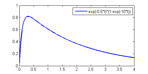
For each of the envelopes, I used exponential functions, such that:
envelope =
  Ao * e(-dk_rate*t) * (1-e(-attack_rate*t))
These exponential functions are compactly calculated at each time step as first-order differential equations, requiring one multiply each, if the decay and attack rates are specified as the fractional change in amplitude per decay sample. So a slow rate of decay would be 0.999 and a fast rate 0.005. A fast rise would be 0.0 and a slow rise 0.99. This is based on a Euler approximation of the first order differential equation:
(y(n) - y(n-1))/dt = -K*y(n-1) with y(0)=Ao and K the decay rateRe-arranging gives
y(n)/y(n-1) = 1-K*dt = R with 0≤R<1 (because K*dt<1 for Euler approximation), so we can just compute y(n)=y(n-1)*RNote that for significant amplitude, you need the attack time to be shorter than the decay time, unless you add some 'sustain' time, which holds the amplitude at full output level for a set time, then lets it decay.
Example:
All arithmetic is done in 16:16 fixed point for good accuracy and speed. The 32-bit fixed notation gives enough dynamic range so that the algorithm does not dither in the range of the DAC. The macros for fixed point are given on a separate page and in the code below. The oscillators are implemented as Direct Digital Synthesis units, accessing a 256 entry sine table. The output is to one channel of a stereo 12-bit SPI attached DAC. (code, ZIP of project). About 5-10% of the cpu is used to generate one FM synth channel, depending on which ISR operations are executing (at opt level 1). This was measured by toggling an i/o pin in the ISR. A separate program just outputs to damped sine waves to the stereo DAC channels. All programs use Protothreads to control execution.
| example | F_main | F_fm | Attack_main | Attack_fm | DK_main | DK_fm | depth_fm | Sustain time |
|---|---|---|---|---|---|---|---|---|
1 |
3 |
0.001 |
0.001 |
0.98 |
0.80 |
2.2 |
0.0 |
|
0.5 |
0.8 |
0.001 |
0.001 |
0.99 |
0.90 |
1.5 |
0.0 |
|
.25 |
0.37 |
0.005 |
0.005 |
0.98 |
0.98 |
2.0 |
0.0 |
|
261 |
783 |
0.99 |
0.95 |
0.98 |
0.97 |
3.0 |
1.0 |
A FM version with 8 predefined timbres plays a pentatonic scale. There is a simple command structure that lets you set:
- timbre 0-7;
- tempo 0-3 ; 8/sec to 1/sec
- play a note; 0-7; C4, D4, E4, G4, A4, C5, D5, E5
- play a scale
The Karplus-Strong Algorithm (KSA) for plucked string synthesis is a special case of the digital waveguide technique for musical instrument synthesis. The KSA is particularly well suited for implementation on a microcontroller, and was originally programmed on an Intel 8080! The simplest version hardly needs fixed point arithmetic, but better approximations do require some more sophisticated digital filters. The basic algorithm fills a circular buffer (delay line) with white noise, then lowpass filters the shifted output of the buffer and adds it back into itself. The length of the buffer (along with an allpass fractional tuning filter and the sample rate) determine the fundamental of the simulated string. The type of lowpass filter in the feedback determines the timber. Prefiltering the white noise before loading the buffer changes the pluck transient timber.
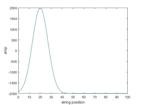
Driving the Karplus-Strong string with a synthesized waveform expands the range of sounds you can make. In this version of the program, the string can be plucked using an initial waveform consisting of noise, sawtooth, triangle or sine wave. It can also be driven by a rising and falling amplitude waveform of all the previous types. In the code, each sample takes around 360 cycles to compute. The KSA output is sent to a SPI-attached DAC. The string length of 76.45 (at 20KHz sample rate) corresponds to approximately note C4 (261.8 Hz). The examples below are generated from the C code. In the table below, the noise examples are Gaussian-distributed white noise, and the Gaussian examples are driven by a exp(-(pluck_position-string_index)2/pluck_width) curve on the string. The bow_rise parameter is the 0 to 100% time in samples to the bow_amp value. The bow_fall parameter is the 100 to 0% time in samples from the bow_amp value to zero amplitude. The wave parameters describe the waveform which is pre-loaded as an initial condition, or driven into the model as a function of time.
(code, zip)
| example | lowpass | damping | pluck_amp | pluck_wave | bow_amp | bow_wave | bow_rise | bow_fall |
|---|---|---|---|---|---|---|---|---|
1 |
0.999 |
1 |
white noise |
0. |
--. |
-- |
-- |
|
1 |
0.99 |
1 |
Gaussian pulse |
0. |
-- |
-- |
-- |
|
1 |
0.99 |
0 |
-- |
0.1 |
white noise |
10000 |
100 |
|
1 |
0.95 |
0. |
-- |
0.1 |
Gaussian pulse |
10000 |
100 |
Solving the wave equation directly (Study Notes on Numerical Solutions of the Wave Equation with the Finite Difference Method, equation 2.15) yields the finite difference form to step the solution forward one sample.

Where un+1 is the displacement at the new time step and i represents the distance along the string. ρ is the propagation speed (range 0 to 1.0 for Courant stability), η is the dissipation which is small (typically 0.001 or so). The actual form of the equation in the code has been modified for efficiency. Most of the multplies have been replaced by shift-add operations. Because η is small, we can Taylor expand and show that
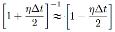
The actual code defines multiply macros using shift and add:
#define times0pt5(a) ((a)>>1)
#define times0pt25(a) ((a)>>2)
#define times2pt0(a) ((a)<<1)
#define times4pt0(a) ((a)<<2)
#define times0pt9998(a) ((a)-((a)>>12))
#define times0pt999(a) ((a)-((a)>>10))
Then uses these macros for the computation. The only full multiplication is by ρ to allow setting the pitch of the string.
for (i=1; i<string_size-1; i++){
new_string_temp = rho * (string_n[i-1] + string_n[i+1] - times2pt0(string_n[i]));
new_string[i] = times0pt9998(new_string_temp + times2pt0(string_n[i]) - times0pt9998(string_n_1[i])) ;
}
memcpy(string_n_1, string_n, copy_size);
memcpy(string_n, new_string, copy_size);