
Introduction to the Project top
For the final project of ECE-5760, we have done a performance evaluation of ARM Cortex-A9 vs FPGA on DE1-SOC board. This project is done using Altera’s OpenCL SDK on DE1-SOC board with a duel embedded ARM core on it.To achieve real time performances from complex algorithms it has become necessary to use massively parallel GPUs or FPGAs along with GPs(General Processors). This heterogeneous computing model is employed in the PC world for graphics, gaming, rendering, server market etc. and now for the handheld/embedded world. To program such systems, Open Computing Language (OpenCL) an open, royalty free standard for parallel programming of modern processors, has been developed. It greatly improves speed and responsiveness for a wide spectrum of applications in numerous market categories from gaming and entertainment to scientific and medical software.
This project is mainly done in OpenCL and C++, where all the kernels are written in OpenCL and host code running on the ARM in C++. Our project aims at evaluating the speedup achieved on FPGA for parallel operations and the overhead involved in achieving that. We have particularly targeted two types of filters to do this evaluation. The Altera OpenCL SDK allows a programmer to use high level code to generate an FPGA design with low-power consumption and good performance. Altera’s AOCL compiler is used to compile the Kernel code to FPGA design and automatically generates SystemVerilog code for the developer. The reasoning behind using filters as the benchmark for OpenCL is because filtering is one of the most important component in image processing applications and computer vision algorithms. Our evaluation aims at comparing the performance of Gaussian Filter and Bilateral filter, which is a nonlinear filter, on ARM and FPGA with the same alignment and memory restrictions.
High Level Design top
OpenCL
The OpenCL standard inherently offers the ability to describe parallel algorithms to be implemented on FPGAs, at a much higher level of abstraction than hardware description languages (HDLs) such as VHDL or Verilog. Although many high-level synthesis tools exist for gaining this higher level of abstraction, they have all suffered from the same fundamental problem. These tools would attempt to take in a sequential C program and produce a parallel HDL implementation. The difficulty was not so much in the creation of a HDL implementation, but rather in the extraction of thread-level parallelism that would allow the FPGA implementation to achieve high performance. With FPGAs being on the furthest extreme of the parallel spectrum, any failure to extract maximum parallelism is more crippling than on other devices. The OpenCL standard solves many of these problems by allowing the programmer to explicitly specify and control parallelism. The OpenCL standard more naturally matches the highly-parallel nature of FPGAs than do sequential programs described in pure C.
The creation of designs for FPGAs using an OpenCL description offers several advantages in comparison to traditional methodologies based on HDL design. Development for software programmable devices typically follows the flow of conceiving an idea, coding the algorithm in a high-level language such as C, and then using an automatic compiler to create the instruction stream. This approach can be contrasted with traditional FPGA-based design methodologies. Here, much of the burden is placed on the designer to create cycle-by-cycle descriptions of hardware that are used to implement their algorithm.
The traditional flow involves the creation of data-paths, state machines to control those data-paths, connecting to low-level IP cores using system level tools (e.g., SOPC Builder, Platform Studio), and handling the timing closure problems since external interfaces impose fixed constraints that must be met. The goal of an OpenCL compiler is to perform all of these steps automatically for the designers, allowing them to focus on defining and optimizing their algorithm rather than focusing on the tedious details of hardware design. Designing in this way allows the designer to easily migrate to new FPGAs that offer better performance and higher capacities because the OpenCL compiler will transform the same high-level description into pipelines that take advantage of the new FPGAs. One of the reasons behind this is because OpenCL is device independent, the programmer simply specifies the device that will be used on the host side, and the compiler will automatically optimize the code for that device. Figure 1 shows an overview of how the system is connected.
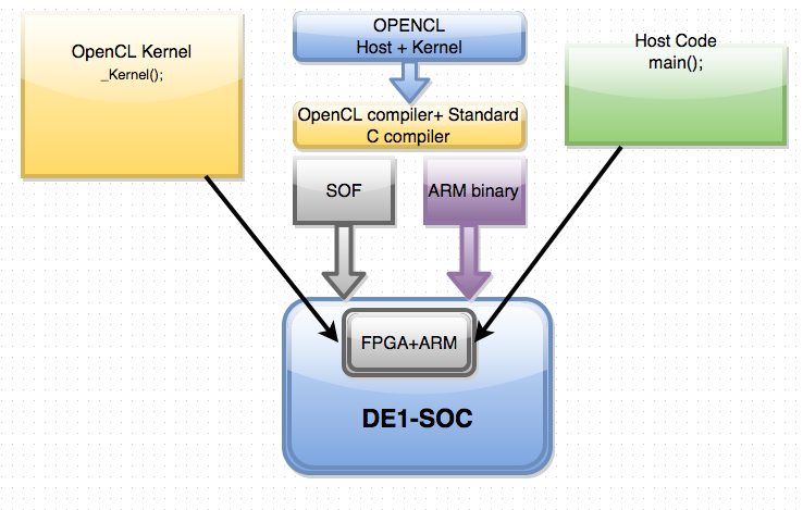
Fig 1.Block Diagram of the Overall Setup
Down the middle of figure 1, we see the various compilers. The Altera OpenCL compiler generates an SOF file that is used to specify the specific hardware configures that the FPGA needs to use. This file contains all the place and route information. The standard C compiler generates the binaries that will run on the host.
As figure 1 shows, DE1-SOC board with FPGA+ARM core is the board used in this project. The host can be written in C++, C to configure the OpenCL Kernel. There are 6 data structures that the host manages; the first of which being the platform. The platform is used to identify vendors implementation of OpenCL. It gives a way to identify a way to access the device. The device is the hardware that the kernel will run on, for the course of this project that device is an FPGA. One OpenCL program is not limited to one device; multiple devices can be run using the same host code to achieve large scale parallelism. The next key data structure the host is responsible for is the program. The program container is used to hold a list of kernels. Kernels are the specific functions or algorithms that will be ran, this is usually the computationally intensive task that is required to be ran. The kernel is also device independent, meaning that it can be ran on any device the that has OpenCL support(GPU’s, CPU’s, FPGA’s). The next big data structure is the command queue. It is the primary source of communication between the host and the device, the host sends the kernels that need to be ran to the command queue to get queued up to be executed. The last vital data structure is the context, which is used to manage the connected devices. Figure 2 shows all of the various data structures are connected together. The DE1-SoC includes a 16-Kbyte memory that is implemented inside the FPGA. This memory is organized as 16K x 8 bits, and spans addresses in the range 0x08000000 to 0x08003FFF
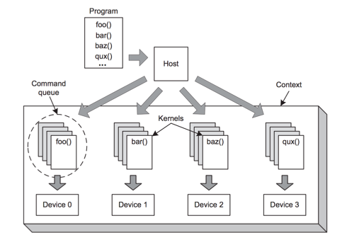
Fig. 2 Device Management using Context Switching
One of the key aspects of using OpenCL is the ability to parallelize tasks. An OpenCL kernel is executed via an array of work items, and all work items run a copy of the same code. Each individual work item is also assigned its own ID, which it can use to index a specific chunk of memory to run its computation on.
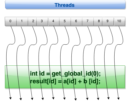
Fig. 3 Basic thread layout
Figure 3 shows how one work item is used to execute data independent operations in parallel via global ID. Several workgroups can be created that encompass these work items as shown in figure 4. OpenCL can divide the monolithic work item array into work groups.
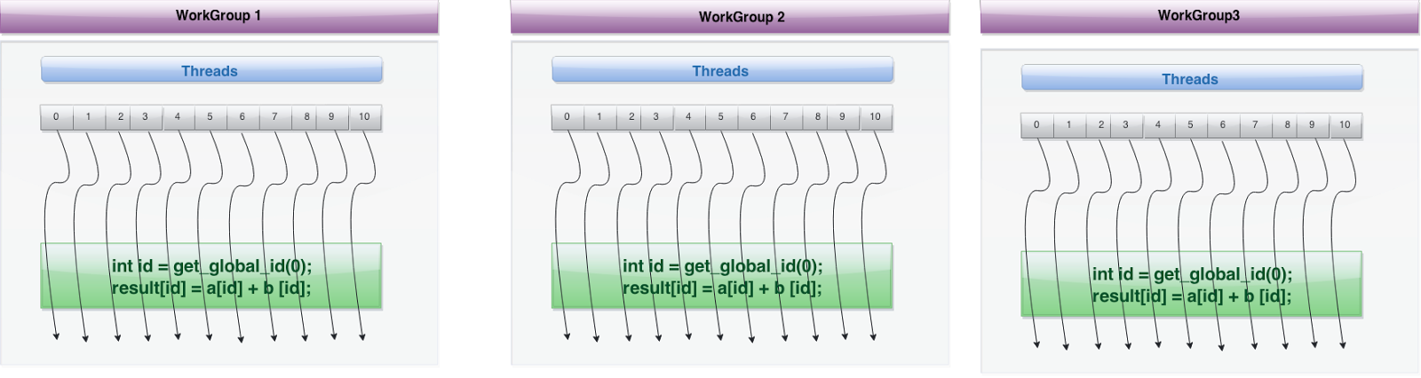
Fig 4. An overview of workgroups
Parallel work is submitted to available devices by launching kernels. The Kernels run over global dimension index ranges (NDRange), broken up into “work groups”, and “work items”. These work items executing within the same work group can be synchronized with each other via barriers or memory fences. The work items in different work groups can’t sync with each other, except by launching a new kernel.
RTL Schematics
This project is done at much higher abstraction level than RTL, and RTL schematic is automatically generated by the tool and compiler. The schematic varies based on the implementation of the design. A high level block diagram which corresponds to logical functionality of the design is shown below. There are two different Kernels which implements two filters. There hardware modules are different from each other and are generated in isolation, but when the main program is run these hardware blocks are instantiated in the design and used for computation.
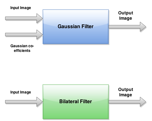
Fig. 5 RTL Level Abstraction
Implementation top
Memory management is one of the most important tasks in any program. Below is a brief explanation of the various ways OpenCL connects the device and host memory.
Memory mapping between ARM and FPGA:
Global memory – It is the main means of communicating reads and writes of data between host and device. Their content visible to all threads but it has long access latency.
OpenCL Device Memory Allocation:
clCreateBuffer() – It allocates objects in the device Global Memory. It returns a pointer to the object and requires five parameters: OpenCL context pointer, Flags for access type by device, Size of allocated object, Host memory pointer, if used in copy-from-host mode, & Error variable.
OpenCL Host-to-Device Data Transfer:
clEnqueueWriteBuffer() - It does memory data transfer to device. It requires nine parameters: OpenCL command queue pointer, Destination OpenCL memory buffer, Blocking flag, Offset in bytes, Sizeof bytes of written data, Host memory pointer, List of events to be completed before execution of this command, & Event object tied to this command.
OpenCL Device-to-Host Data Transfer:
clEnqueueReadBuffer() – It does memory data transfer to host. It requires nine parameters: OpenCL command queue pointer, Source OpenCL memory buffer, Blocking flag, Offset in bytes, Sizeof bytes of read data, Destination host memory pointer, List of events to be completed before execution of this command, & Event object tied to this command.
- A Kernel is invoked once for each work item. Each work item has private memory.
- Work items are grouped into a work group. Each work group shares local memory
- The total number of all work items is specified by the global work size. global and constants memory is shared across all work work items of all work groups
OpenCL Memory Systems-
- Global – large, long latency.
- Private – on-chip device registers.
- Local – memory accessible from multiple PEs or work items. It can be SRAM or DRAM, must query.
- Constant – read-only constant cache.
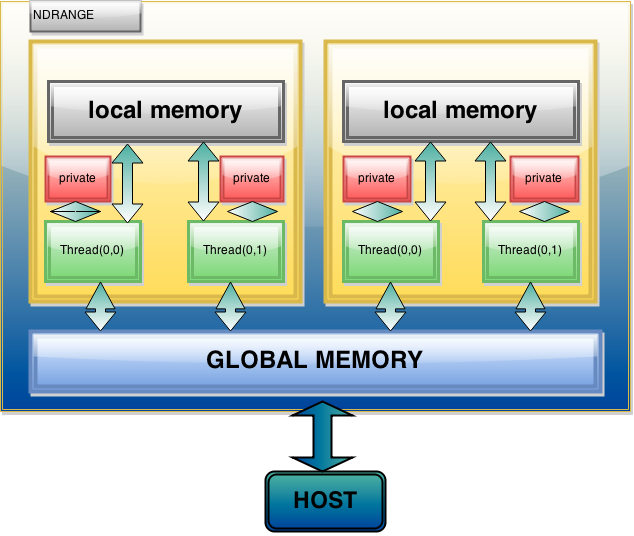
Fig 6. Memory Management System
Filtering
The idea of spatial image filtering is to have a mask or kernel of a certain size that applies a desired operation to the image pixels under the kernel. By moving the kernel around the image, so that all pixels are visited by the center of the kernel, the image is filtered. The operation applied to the underlying image may be either linear or nonlinear. Gaussian filter is a linear filter while bilateral filter is a nonlinear filter. This implies that the filter kernel will be a matrix of coefficients that will be multiplied with the corresponding underlying image pixels. The sum of all products at each location will yield the pixel values of the filtered image.
Linear Filtering with Gaussian Blur (GB): Convolution by a positive kernel is the basic operation in linear image filtering. It amounts to estimating at each position a local average of intensities and corresponds to low-pass filtering.
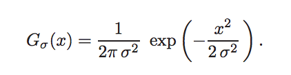
Fig 7. Linear Gaussian Filter
So, Gaussian filtering is a weighted average of the intensity of the adjacent positions with a weight decreasing with the spatial distance to the center position p. This distance is defined by Gσ(||p − q||), where σ is a parameter defining the extension of the neighborhood. As a result, image edges are blurred.
Nonlinear Filtering with Bilateral Filter (BF): Similarly to the Gaussian convolution, the bilateral filter is also defined as a weighted average of pixels. The difference is that the bilateral filter takes into account the variation of intensities to preserve edges. The rationale of bilateral filtering is that two pixels are close to each other not only if they occupy nearby spatial locations but also if they have some similarity in the photometric range. The bilateral filter, denoted by BF[*], is defined by
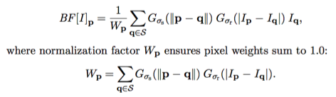
Fig 8. Non-Linear Bilateral Filter
Bilateral filtering is non-iterative, nonlinear and combines domain (spatial closeness) and range (color similarity) filtering. The coefficients of the kernel are computed locally and depend on both variables, thus achieving a good filtering behavior where the pixels’ similarity is high e.g. inside regions. It also preserves areas where similarity is low, e.g. on edges. The bilateral filtering is less content dependent and provides exceptional results with a fixed set of parameters, thus giving highest quality at the lowest computational cost compared to other filters of kind e.g anisotropic diffusion filtering.
Parameters σs and σr will control the amount of filtering for the image. The equation is a normalized weighted average where Gσs is a spatial Gaussian that decreases the influence of distant pixels. Gσr is a range Gaussian that decreases the influence of pixels q with an intensity value different from p. Note that the term range addresses quantities related to pixel values, unlike the term spatial which refers to pixel location.
Parameters- The bilateral filter is controlled by two parameters: σs and σr.
• As the range parameter σr increases, the bilateral filter becomes closer to Gaussian blur because the range Gaussian is flatter i.e., almost a constant over the intensity interval covered by the image.
• Increasing the spatial parameter σs smooths larger features. An important characteristic of bilateral filtering is that the weights are multiplied, which implies that as soon as one of the weight is close to 0, no smoothing occurs. As an example, a large spatial Gaussian coupled with narrow range Gaussian achieves a limited smoothing although the filter has large spatial extent. The range weight enforces a strict preservation of the contours.
Results top

Figure 9. Original Unfiltered Image


Figure 10,11. Gaussian Filtered Image & Bilateral Filtered Image
Filter Iterations (Gaussian Filter) |
FPGA |
ARM |
5 |
2.669 |
10.673 |
10 |
5.344 |
21.348 |
15 |
8.25 |
33.11 |
20 |
10.986 |
42.711 |
25 |
13.814 |
53.387 |
30 |
16.935 |
64.056 |
35 |
19.859 |
74.759 |
40 |
22.84 |
85.4 |
45 |
25.93 |
96.076 |
50 |
29 |
110 |
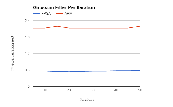
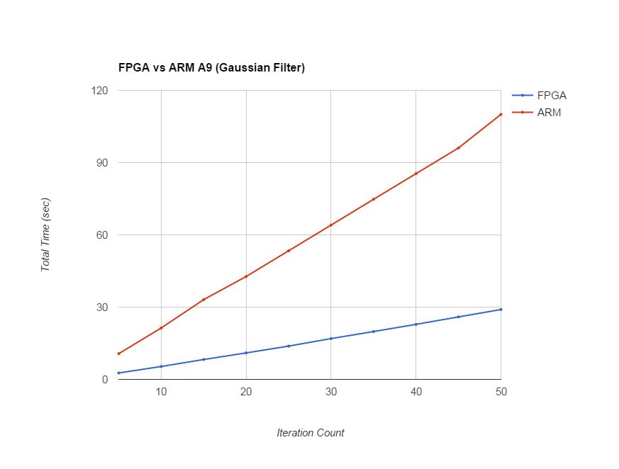
Figure 12,13. Trends for Gaussian Filter Per Iteration & for Total Iterations
Filter Iterations (Bilateral Filter) |
FPGA |
ARM |
5 |
3.154 |
49.628 |
10 |
6.637 |
99.256 |
15 |
10.343 |
153.704 |
20 |
14.208 |
198.571 |
25 |
18.404 |
248.329 |
30 |
22.857 |
307.744 |
35 |
27.567 |
347.648 |
40 |
32.253 |
410.281 |
45 |
37.403 |
447.192 |
50 |
42 |
512 |
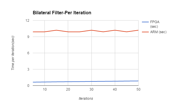
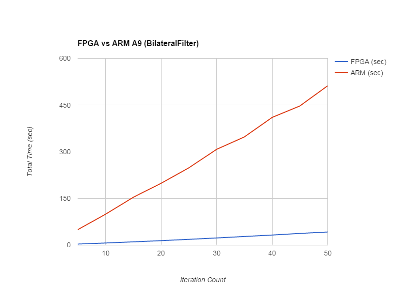
Figure 14,15. Trends for Bilateral Filter Per Iteration & for Total Iterations
The speedup in Gaussian filter on FPGA is 4X as compared to ARM implementation. For bilateral filter, the speedup is 10X. Although speedup on FPGA is usually 10x-100x, it depends upon the algorithm as well as the the amount of parallelism exploited in the hardware. As in case of bilateral filter, there are a lot of floating point operations, all the dedicated DSP blocks are used on FPGA, giving it higher speedup as compared to ARM. The logic utilization is around 51% with all 87 DSP blocks used along with 2 fractional PLLs.
The global work item size as specified in for the parallel execution of the kernel is the image size. The local workgroup size was kept to 64. This means 64 kernels are invoked in each workgroup. This number can be increased to exploit more parallelism, but there is a limit to local memory as a workitems in a workgroup shares the same local memory, while all workgroups shares the same global memory.
Conclusion top
The overall results of the project were as expected, the FPGA outperformed the serial version of the algorithm. The approach that we took for the development of the project seemed optimal at the beginning, however have the knowledge of doing the project, some portions should have been done differently. One of the biggest issues that arose with the project was attempting to get I/O working properly with the FPGA using OpenCL for an optional expansion. Several days were lost researching ways of doing this with OpenCL. Due to the limitations of the libraries available, this task proved to be impossible.
The other issue that emerged during the course of the project was the lack of support to load images on to the FPGA for processing. Even though OpenCL does have structures in its libraries for this task, Altera's OpenCL SDK does not have support for those data structures. However, to overcome this obstacle, the team was able to adapt a BMP library that was obtained from the blog. When this library was introduced, one of the largest issues with the projects was overcome. Other minor challenges arose, but luckily all the tools required to overcome them were available. Overall though, the decision to go with OpenCL to implement the filters was a great learning opportunity for every member of the team. For the future prospects of this project, one interesting analysis would be to implement both filters in Verilog and see how they perform when compared to OpenCL in terms of speed and area.
References top
This section provides links to external reference documents, code, and websites used throughout the project -
OpenCL and FPGA Board
- OpenCL SDK Guide
- Implementing OpenCL with FPGA
- DSP on FPGAs
- Introduction to OpenCL
- More about OpenCL
- OpenCL DE1-SoC Starter Guide
Image Processing
Code Repository
Acknowledgement top
We would sincerely like to acknowledge Dr. Bruce R Land for his overall project guidance and timely smart suggestions which helped us to complete the final project in the provided time frame with required finesse.
We would also like to thank our TA Deepak Awari for helping us in debugging the project whenever required and providing us with useful insights on the project.