Introduction

We designed, implemented, and tested a Frisch-Hasslacher-Pomeau (FHP) cellular automaton, that could be displayed on a 640 * 480 VGA screen. The FHP model, a leap from the traditional HPP model, represents a significant advance in the simulation of gasses and liquids using lattice gas automata.

Our high-performance system, capable of handling nearly 2 million particles, offers a captivating exploration into the microcosmic world of particles. We have six directions for particle motion, four diagonal and two horizontal directions, which added much complexity to the system.

To increase interactivity, we've included a pause button and configurable initial states. Users can freeze the simulation at any point, allowing for detailed analysis and appreciation of the complex patterns that emerge. We also provide functionalities of changing the initial directions of the particles, leading to distinct system behavior and visual effects, and all of them can be conveniently selected by switches.

We hope that our FHP model project is a scientific and artistic masterpiece, serving as an engaging, therapeutic, and educational platform. We invite users to dive into this fascinating world of particles and uncover the beauty of its emergent patterns.

High Level Design

The Frisch–Hasslacher–Pomeau (FHP) model is a type of lattice gas automaton, a class of cellular automata used to simulate fluid dynamics. It was first introduced by U. Frisch, B. Hasslacher, and Y. Pomeau in 1986 as an improvement over the earlier Hardy-Pomeau-de Pazzis (HPP) model. The FHP model utilizes a hexagonal lattice, which is a better approximation to isotropy than the square lattice of the HPP model. Each intersection on the lattice can be thought of as a cell that can contain particles. These particles can move to neighboring cells along the six directions of the hexagonal lattice.

One of the main features of the FHP model is its use of collision rules. When two or three particles meet at a cell, they will interact and change directions. The rules ensure that both the number of particles and momentum are conserved, reflecting the conservation laws of real physical systems.

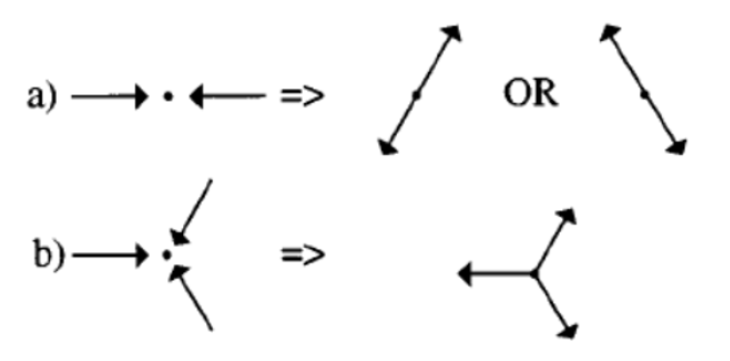
Two rules governing the movements of particles in FHP model.

FHP models are particularly useful for simulating fluid flow, including phenomena like shock waves and turbulence. They can be used in a variety of fields, from physics to engineering and computer science.

The simplicity of the rules, combined with the complex behaviors that emerge from them, make the FHP model a powerful tool for understanding fluid dynamics. While the model is not without its limitations, it has been foundational in the development of lattice gas automata and the broader field of computational fluid dynamics.

We try to implement the FHP algorithm based on the Python, and here is the core code about the collision and propagation below:

            
              def collision_phase(self) -> None:
                for x in range(self.w):
                  for y in range(self.h):
                    a, b, c, d, e, f = self.a[x][y], self.b[x][y], self.c[x][y], self.d[x][y], self.e[x][y], self.f[x][y]
    
                    tb_ad = (a & d) & (~(b | c | e | f))
                    tb_be = (b & e) & (~(a | c | d | f))
                    tb_cf = (c & f) & (~(a | b | d | e))
    
                    triple = (a ^ b) & (b ^ c) & (c ^ d) & (d ^ e) & (e ^ f)
    
                    rnd = random.getrandbits(8)
                    no_rnd = ~rnd
    
                    cha = (tb_ad | triple | (rnd & tb_be) | (no_rnd & tb_cf))
                    chb = (tb_be | triple | (rnd & tb_cf) | (no_rnd & tb_ad))
                    chc = (tb_cf | triple | (rnd & tb_ad) | (no_rnd & tb_be))
                    chd = cha
                    che = chb
                    chf = chc
    
                    self.K_a[x][y] = a ^ cha
                    self.K_b[x][y] = b ^ chb
                    self.K_c[x][y] = c ^ chc
                    self.K_d[x][y] = d ^ chd
                    self.K_e[x][y] = e ^ che
                    self.K_f[x][y] = f ^ chf
            
          

            
              def propagation_phase(self) -> None:
              for x in range(self.w):
                for y in range(self.h):
                  # Propagation with wall conditions
                  self.a[x][y] = int(self.K_a[x][(y - 1)]) if y > 0 else int(self.K_d[x][y])
                  self.b[x][y] = int(self.K_b[(x + 1)][(y - 1)]) if x < self.w - 1 and y > 0 else int(self.K_e[x][y])
                  self.c[x][y] = int(self.K_c[(x + 1)][(y + 1)]) if x < self.w - 1 and y < self.h - 1 else int(self.K_f[x][y])
                  self.d[x][y] = int(self.K_d[x][(y + 1)]) if y < self.h - 1 else int(self.K_a[x][y])
                  self.e[x][y] = int(self.K_e[(x - 1)][(y + 1)]) if x > 0 and y < self.h - 1 else int(self.K_b[x][y])
                  self.f[x][y] = int(self.K_f[(x - 1)][(y - 1)]) if x > 0 and y > 0 else int(self.K_c[x][y])
            
          

The result is shown in the following animation:

Result of FHP based on Python

Hardware Design

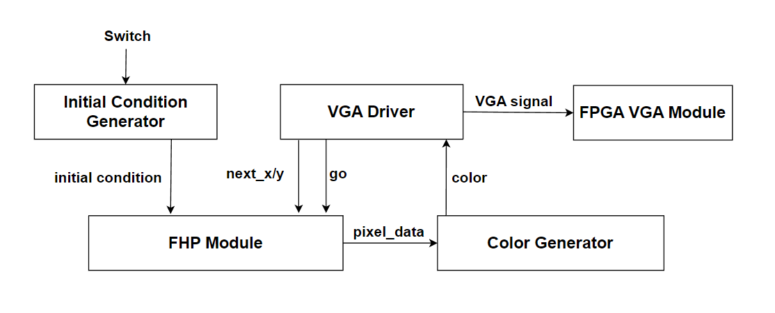
Block Diagram of Top Level Design

For top level module, we use switches as inputs to control the initial conditions and system behavior. Specifically, the switches are used in the following way:

• SW[0] is the FHP reset switch, it sends the reset signal to the FHP module to revert back to the initial conditions.
• SW[6:1] represent 6 bits for the initial conditions. Each bit represent one of the six possible directions of a particle at a certain pixel location. This value will be passed into the FHP modules and will be written into the memory location corresponding to every pixel location within the initialization boundary.
• SW[7] stretches the initial boundary horizontally to 640 pixels.
• SW[8] stretches the initial boundary horizontally to 480 pixels.
• SW[9] pauses VGA animation and FHP computation, so that users can analyze closely what is going on.

After the initial conditions are fed into the FHP module, it reads the next_x, next_y location from our customized VGA driver, and the go signal which comes at 30hz for a stable refresh rate. The colors to be passed into the VGA driver, are fetched from a color generator. The color generator takes in the 6-bit representation at a pixel location, and translate that to 8-bit color with gradient color changes to reflect the density at such location. Finally the VGA signal will be written to the FPGA VGA module and will be displayed on the screen. Following are details of each module in our implementation.

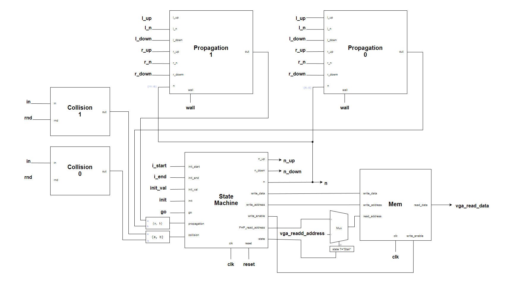
Our FHP module consists of 319 column modules, where all the column modules are identically generated except for the column 0 and 319 as they have different boundary conditions. A rand module is in charge of generating random values for all the columns. The output is selected by using the next_x signal to output the corresponding VGA signal vga_read_data.

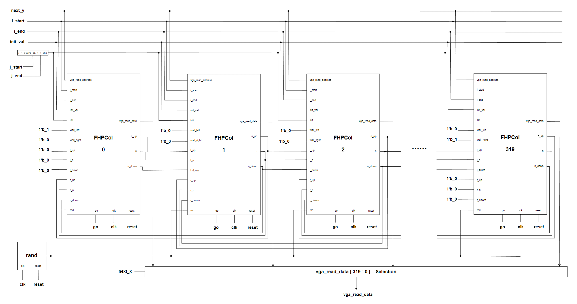
Block Diagram of FHP

For all the FHP columns, we assign the following inputs identically:

• vga_read_address is the next_y requested by the top level module.
• i_start, i_end, which are the initial conditions boundary. It determines the vertical size of the initial particle region.
• init_val is the initial condition vale for each particle to be written into the M10k memory. Each one of the six bits in its value represent a particle moving towards a certain direction. The initial condition value is controlled by the switches in the top level module.
• init is a flag that determines whether a column should fill in initial values or keep them empty. It is determined by the j_start and j_end inputs for the FHP module. Only the columns in between j_start and j_end will be assigned init=1, which indicates they will be loading in initial conditions.
• l_up, l_n, l_down, stand for left up, neighbor, and down. These values will be fetched from the left column module (if exist) for collision and propagation calculation purposes. Boundary conditions will be set to 0.
• r_up, r_n, r_down, stand for right up, neighbor, and down. These values will be fetched from the right column module (if exist) for collision and propagation calculation purposes. Boundary conditions will be set to 0.
• wall_left, wall_right are boundary conditions, Only col_0 has wall_left=1, and only col_319 has wall_right=1.

For the random module, we used Bruce’s 16-bit parallel random number generator. Which generates 64 bits for pseudo-random values. We split these random bits and each column will randomly get one bit from the sequence.

Details of FHPCol

In our FHPCol module, we are implementing the design of a single column, which consists of two vertical pixel rows to be displayed on the VGA screen. The module itself includes a state machine, and it further instantiates two collision modules and two propagation modules, which are the two most important parts in our design. It also instantiates a Mem module in order to access data.

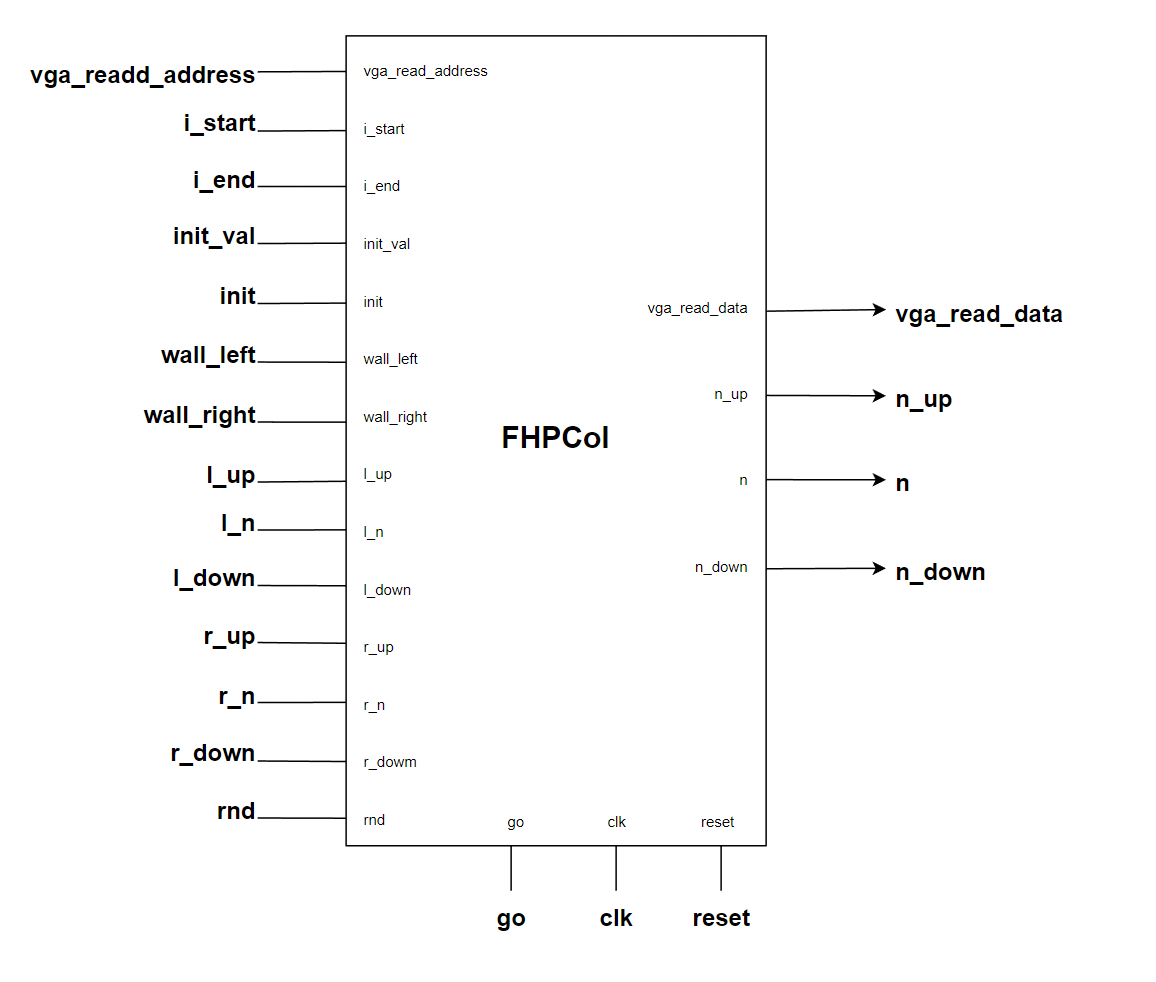
Block Diagram of FHPCol

To start with the state machine, two states are essentially the core of our design: collision and propagation, while we also have necessary initial and stall states in between. The collision state updates the collision outcomes for each pixel and the propagation stage actually moves the particles towards its current direction for one step.

• On reset, we clear the write_addr, write_data, write_enable registers so that we can start from the initial memory location (row 0) for computation.
• In the initial state, if the init value is set to 1, we compare the input i_start, i_end, which regulates the boundaries of the initial particles with the write_addr value to check if the current memory address needs to be filled with initial conditions. init_val will be used as the value to be written into the M10k memory if the current address is within the initialization boundary. After reaching the bottom row, we transition to the next state. (stall)
• In the stall state, we simply wait for a signal go, otherwise we keep resetting the read and write address to 0 to prepare for the next stage. (collision)
• In the collision state, we provide incrementing addresses for reading and writing memory. The FHP_read_addr will be fed into the two collision modules, so that they could access a pixel location and calculate the collision outcomes. The write_addr will be used to write the outputs from two collision modules c_node_1_out and c_node­_0_out to the corresponding pixel location. We exit this state when we reach the bottom and enter the next state. (propagation)
• In the propagation state, our state machine behaves very similarly. We would need to consider boundary conditions now since we need to deal with moving particles and they could be heading towards the wall. We check the boundaries by comparing the write_addr with the parameters of top and bottom row, and change a wire wall­_0 accordingly to let the propagation modules know that there is a wall condition. The wire is a 4-bit representation since we have different expected propagation behaviors when particles hit the wall from different directions. Other than the wall condition check, the propagation state simply updates the read and write address in each clock. The inputs l_up, l_n, l_down, r_up, r_n, r_down are essentially the neighboring particles and will be fed into the input of propagation modules. We write the output of the two propagation modules into the M10k memory each clock. When we are done, go back to the stall state.

Details of the collision, and propagation module will be discussed in subsequent paragraphs.

In our Collision module, we are implementing the change of direction of particles after a collision under different conditions. It has two inputs and one output displayed below.

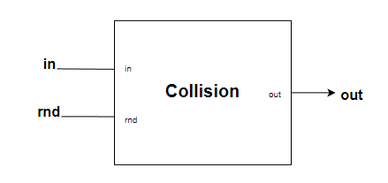
block Diagram of Collision

The inputs are a 6-bit vector in, which represents the states of the six directions of a cell in the hexagonal lattice (a-f), and a single bit rnd, which appears to be a random bit used in certain collision rules. The output is a 6-bit vector out, which represents the states of the cell after the collision.

And we have three variables 'ad', 'be', 'cf' to determine whether two particles have collided. For instance, when a particle collides with a particle nearby along the 'ad' direction, the values of in[0] and in[3] are both 1, while others are 0. The variable 'triple' represents a three-particle collision.

The collision rules are encoded in the definitions of the cha to chf variables. A direction changes state if there is a two-particle collision along that direction, a three-particle collision, or a two-particle collision along one of the other pairs of directions, depending on the value of rnd.

Finally, the states of the cell after the collision are calculated by XORing the initial states with the corresponding change variables. These are then concatenated into the out variable.

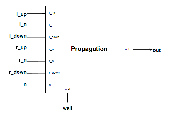
block Diagram of Propagation

This module named Propagation demonstrates the propagation step of the FHP model, where particles move to neighboring cells based on their current directions, with the presence of walls altering their paths. This step, along with the collision step, allows the simulation of complex fluid dynamics with the FHP model. It has multiple inputs and one output.

The inputs are six 6-bit vectors (l_up, l_n, l_down, r_up, r_n, r_down, and n) representing the states of the neighboring cells in the hexagonal lattice, and a 4-bit vector wall representing the presence of walls in the four cardinal directions.

The output is a 6-bit vector out representing the states of the cell after the propagation. The variables a to f represent the current state of the cell. The variables a_in to f_in represent the incoming particles from neighboring cells. The variables w_u to w_r represent the presence of walls in the four cardinal directions, and nw_u to nw_r represent the absence of walls. The propagation rules are encoded in the definitions of the aout to fout variables. Each direction propagates the incoming particle if there is no wall, or a particle from another direction if there is a wall.

Let's take the example of a particle transforming to direction a. According to the code "aout = (((nw_r & nw_d) & a_in) | (w_d & c) | (w_r & f))", here is a breakdown of this line:

• ((nw_r & nw_d) & a_in): This checks if there are no walls to the right (nw_r) and down (nw_d). AND if there is an incoming particle from the right and down (a_in). If all these conditions are true, a particle will propagate into the current cell from the "a" direction.
• (>w_d & c): This checks if there is a wall down (w_d). AND if there is a particle in the "c" direction. If these conditions are true, the "c" particle cannot propagate down due to the wall, and instead propagates in the "a" direction.
• (w_r & f): This checks if there is a wall to the right (w_r) AND if there is a particle in the "f" direction. If these conditions are true, the "f" particle cannot propagate right due to the wall, and instead propagates in the "a" direction.

Results & Conclusion

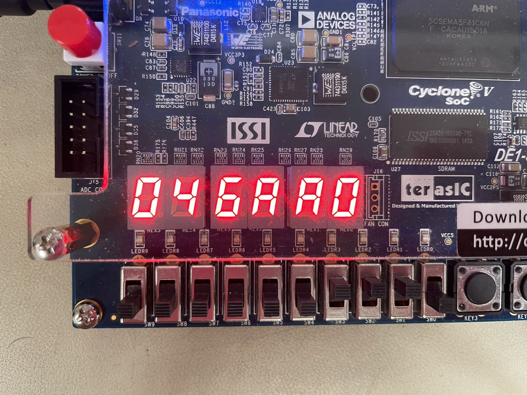
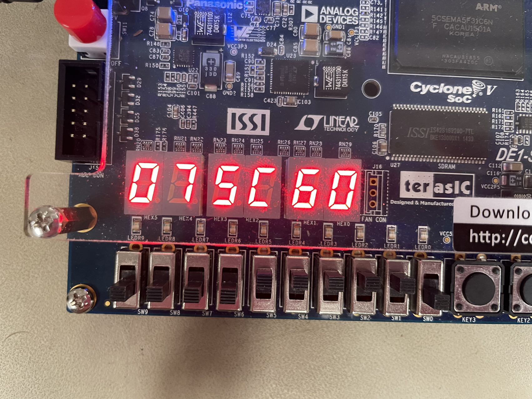
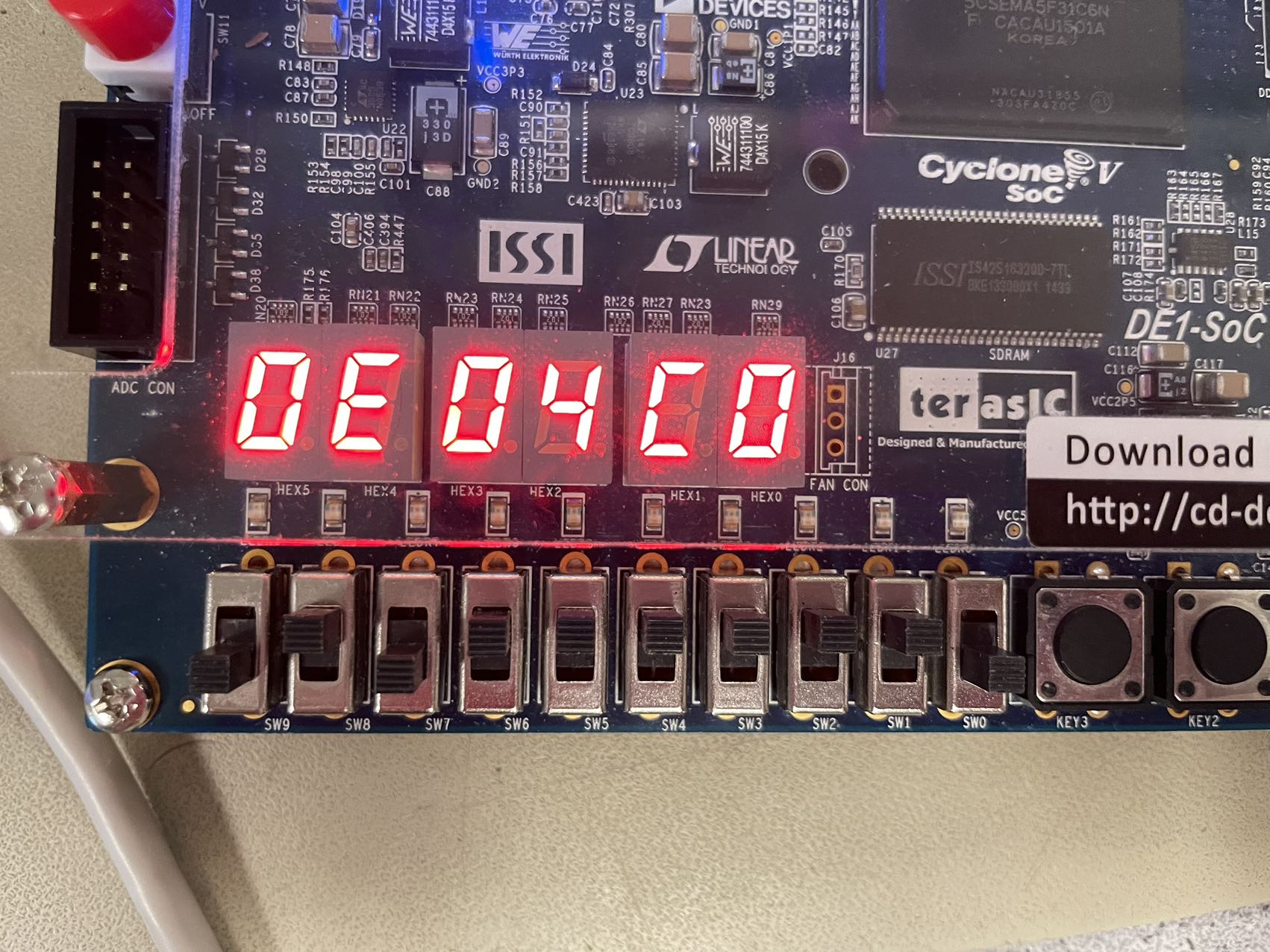
By completing this final project, we created a particle system that was able to simulate at maximum 1.8 million particles at 30 Hz. The implementation was done by using 320 parallel computation modules for the collision and propagation of each particle. We included customization features such that the user will be able to pause the animation or adjust initial conditions of the system, which will eventually lead to very different system behaviors. Compared to our prototype implementation, which was in python, our FPGA implementation showed significant improvement in performance: the python implementation took ~30 mins to animate 300 frames, which is equivalent to 10 seconds of animation at 30 Hz; Our FPGA was able to animate in real time at 30 Hz with stalling, and we may be able to achieve higher frame rates by reducing the stalling. Following are some demonstration videos of our particle system, and screenshots of the particle number displayed in Hex format.

• When we set S[1], S[2], S[3] as high, the number of particle and the effect displayed below:

• When we set S[1], S[2], S[3], S[4], S[5] as high, the number of particle and the effect displayed below:

• When we set S[1], S[2], S[3], S[4], S[5], S[6] as high, the number of particle and the effect displayed below:

In these demonstrations, we can see that different initial conditions and particle directions will lead to very different system behavior. Generally, we will be expecting both vertical and horizontal density waves oscillating between both sides of our screen. Over time, the system will become closer to a state of equilibrium where all the particles are distributed evenly across the screen. However, due to the randomness and the complexity of the model we have implemented, there will always be various types of smaller oscillations that we can visually observe in certain regions of the screen, which changes from time. It would definitely be more interesting to add more obstacles into this project, but due to our current design and resource utilization, we were not able to add such features within the time limit.

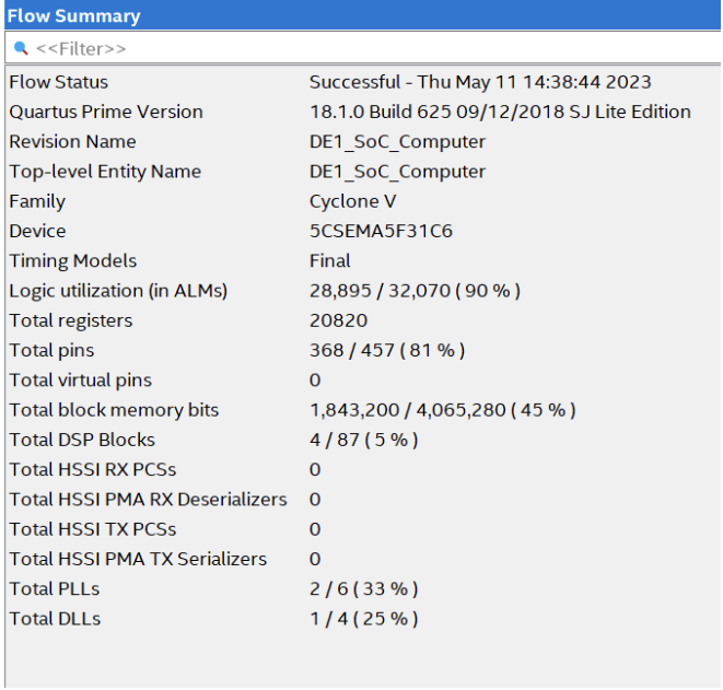
FPGA Resource Utilization

The flow summary shows that we have used 90% of the logic, 81% of total pins, and 45% of the memory. We initially thought memory might be the constraint but it turned out to be the logic. Currently we have stall stages which holds our animation at 30Hz, and we should be able to animate the particles at 60Hz without changing the logic utilization by. However, to further upscale it to a higher resolution, or to implement more complicated models, we might not be able to meet the resource constraints without modifying the current program architecture.

The Chip planner shows more details of the resource utilization.

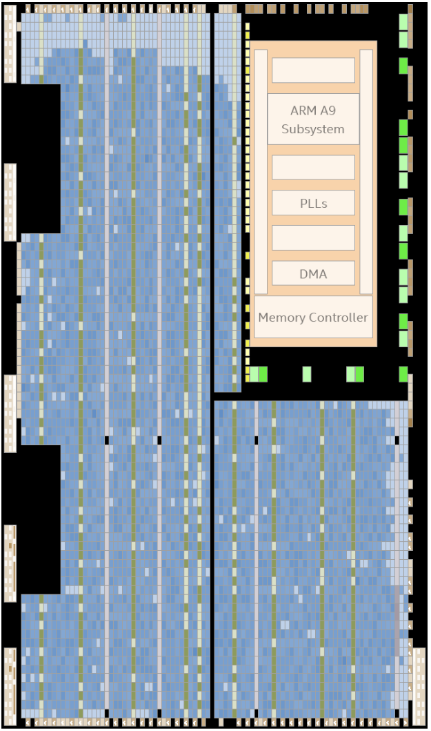
Chip_Planner

In this project, we have built a FHP particle simulator on a 640 * 480 VGA screen. With each pixel holding at most 6 particles, we can achieve at most ~1.8 million particles over the entire screen. Since more particles are represented than the number of pixels, we chose to represent the density in 6 different colors to make it visually more intuitive. We simulated this project at 30Hz, and we implemented switch controls for changing various initial condition parameters.

Following are some features that we may be able to achieve if given more time:

• Add/remove obstacles to add complexity to the simulation area
• Add/remove particles so that users can interfere when the system is close to equilibrium
• Animate the system at 60Hz – this shouldn’t involve much design change, we just need to verify that our current computation modules are faster than or equal to 60Hz.
• Displaying more info on a corner of the screen - maybe we can shrink the animation area a little to save some resource utilization, and trade that for more complex features as previously mentioned.

A lot of parts of our design/architecture were inspired by the Mandelbrot lab and the Drum lab. They have been surprisingly useful when we were considering ways of parallelization. Many thanks to Hunter and Bruce for the abundant resources and documentation!

Appendix

The group approves this report for inclusion on the course website.

The group approves the video for inclusion on the course youtube channel.

Course Website

Random Number Generator

Previous 5760 project on HPP

VGA driver

FHP Collision model

Kailing: Architect, RTL Designer, Design Verification Engineer, Documentation

Zechen: Software Engineer, Design Verification Engineer, Documentation

Ziyuan: Design Verification, UI/UX Designer, Documentation