Results and Discussion

The code as provided for download at the link on the left, allows for five different input variables.  These are in same order as used as arguments in the code:
           n -                     The size of the population to be tested
           hidden -              The number of hidden units each ant has
           mFactor -             The mutation factor, i.e. after each round the offspring will be mutated by a
                                      random number chosen from +/- mFactor
           selectiveStrength -defines what fraction of the population is kept for the generation of the next
                                     offspring, i.e. a selective strength of 0.2 means the top 20% of the generation
                                     get to produce offspring for the next generation
           cycles -                The number of evolutionary cycles the program should run for

Simulation 1 - How many evolutionary cycles does it require to converge to a solution?

Simulation 1 was run using the following parameters
            n = 10 000
            hidden = 5
            mFactor = 0.2
            selectiveStrength = 0.2
            cycles = 20

In all simulations it is worth noting that only a small fraction (generally less than 1%) achieved an evolutionary fitness (i.e. the number of food found on the track) of higher than 0.  Therefore in the following figure the number of non-zero ants in the population of 10 000 is shown as well as the mean fitness of these elements:

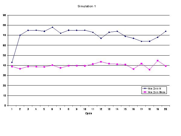
This graph shows that the number of ants that can evolve from a random population at a mutation strength of 0.2 appears to level off after as few as 2-3 cycles.  Taking a histogram of the data at each time point reveals a similar result: movie.  It is important to note here that only the non-zero data is graphed.  This can decrease the non-zero mean as well when more 'ants' move up from 0 to the low range of fitness and therefore a graph of overall mean fitness versus evolutionary cycle is more informative:



















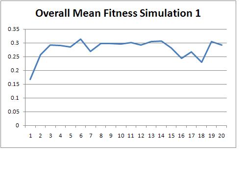
Again, one can see clearly that while there is a drastic change after the first and second cycle, the overall fitness mean levels off quickly after the third cycle.  Similarly the maximum fitness (in this case it was 81) was generally reached by the third evolutionary cycle in this simulation and others.  Thus, for all remaining simulations a cycle number of 10 was considered sufficient.


Simulation 2 - What happens if you change the number of hidden units?

The second simulation tested different number of hidden units and how this would affect the overall mean fitness and the maximum fitness in the final population.  The parameters used were:

            n = 10 000
            hidden = between 1 and 10
            mFactor = 0.2
            selectiveStrength = 0.2
            cycles = 10

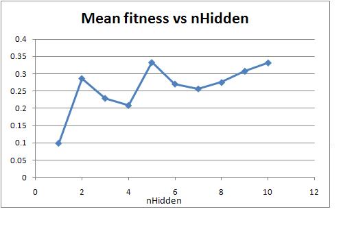
The results are summarized in the graphs below:

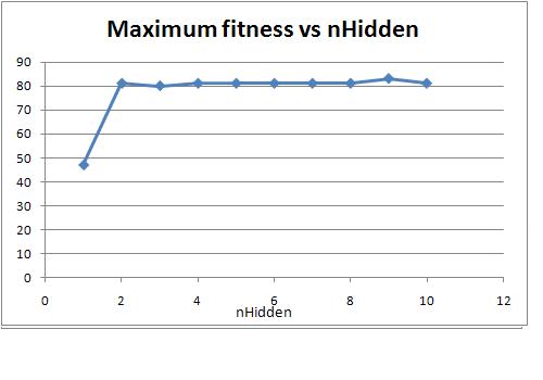
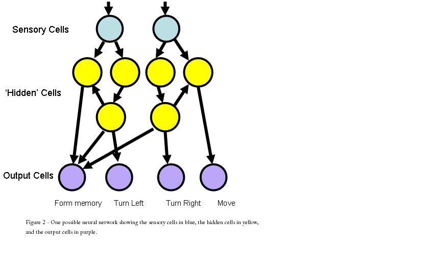
What was particularly interesting about this simulation was that with only one hidden unit a single event was witnessed where the maximum fitness was  76, which is suprisingly close to the overall maximum fitness witnessed of 83.  The neural circuitry of this 'ant' is shown below:


























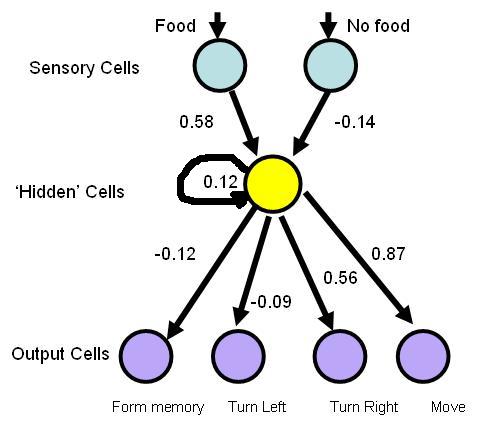
This circuitry resulted in a very efficient algorithm that if there was food in front of the ant, it would move forward, and if there was no food, it would alternate between moving forward 1-2 times and turning right 3-4 times.  This appears strange at first, as the no food sense with a synaptic connection of -0.14 should not trigger any response.  However, it is important to remember that as the ant traverses the trail each unit has a memory of its state.  The ant if (and only if) it starts out with food in front of it, will (as with our trail) build up close to a state level of 1 before it doesn't see any food.  In this case, while its state is reduced by -0.14, it is still above threshold (0.7) and activates the outputs.  Though in some cases it may take more than one time step before any output is above threshold and that is when both the turn right and the move forward get activated simultaneously.  In this case however, the code checks the turn right first and if that is activated decides on that path of action.  Thus, taking advantage of nearly 'loop holes' in the code, the evolutionary algorithm has produced a very efficient single hidden unit ant for tracking trails.

In general though, one can see from the graphs that the maximum of above 80 fitness is quickly reached at 2-3 units, a small optimum appears to occur at 5 units and after which the increase in mean fitness is only minimal.  The computer used for modelling unfortunately was not able to support simulations above 10 hidden units and would throw an out of memory error, however given the data one can assume that the increase in fitness would not have been drastic.

Simulation 3 - How does the mutation factor affect the maximum and mean fitness?
The third simulation tested different mutation factors and how this would affect the overall mean fitness and the maximum fitness in the final population.  The parameters used were:

            n = 10 000
            hidden = 5
            mFactor = between 0.1 and 5
            selectiveStrength = 0.2
            cycles = 10

The results are summarized in the graphs below:




































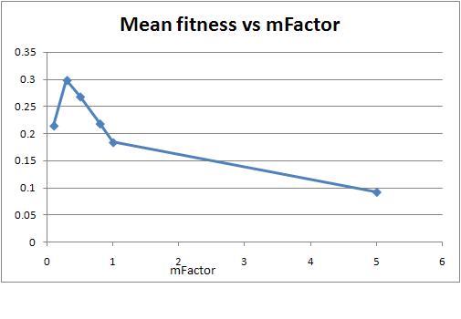
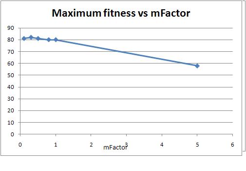
The results of this simulation is very much as expected.  A too low or way too high mutation factor does not lead to a good evolutionary algorithm.  The optimum as can be seen from the graphs, appears to be around 0.2-0.4.  It is also good to see that at very high mFactors (=5), the mean and maximum fitness drop strongly, verifying that our evolutionary algorithm is functioning correctly and producing significantly stronger results than a simple random trial and error.