Skin Detection
 Detecting the skin was the most challenging part in this lab. We initially used a sample position and determined its RGB values and accordingly set the threshold for skin detection. However this method was not robust as it would get affected by the lighting conditions. Under improper lighting, the RGB values would be very low and thus the module wouldn't detect our hand. We searched for couple of algorithms online for skin detection. We found many methods, using HSL (Hue, Saturation, Lightness), or by using Normalized RGB, or by using YCbCr ( Luma, Blue-difference, Red-Difference). However the most simplest and yet effective one was by using normalized RGB values.
In this method, instead of using the actual RGB values, we divide each value with the total R+G+B value, thus normalizing it.
R/(R+G+B)
G/(R+G+B)
B/(R+G+B)
Thus even if due to lighting variations, if the RGB values change, these normalized values will not change much and hence we would still be able to detect the skin by giving appropriate threshold conditions.
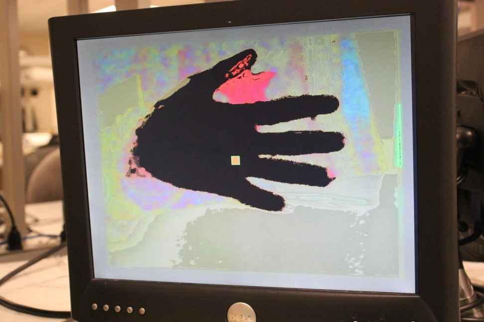
First in order to set threshold conditions we should capture appropriate sample values. We created a small green box at the center of the screen that would calculate the average RGB values of all the pixels inside it. This average RGB value would be our sample value. Setting SW[12] gets the block to be displayed on the screen. Thus we can just put our finger inside this box and press KEY2. Pressing KEY2 will capture our sample value and detect all the pixels that are close to this sample. We can thus detect any skin tone since before every detection we take a sample. Not only can our module detect just skin, but any other specific colour too. All we need to do is set the sample initially as needed. All this is included inside the detect_control module.
Keyboard generation for piano and drum
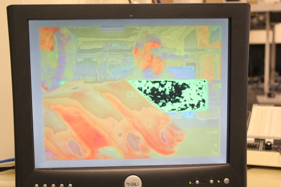
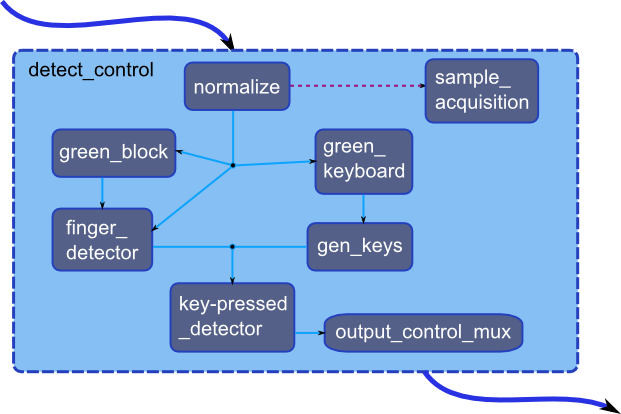
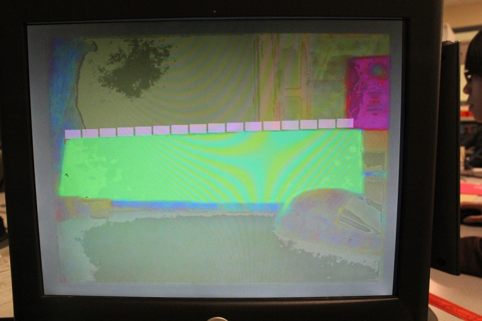 We created a layout of piano and drum notes on a green chart paper. For piano we used 16 notes and for drum we used 5 notes. We created modules inside the detect_control module to detect this paper and plot the keyboard on the VGA screen. This module looks for only green colour. The corners of the chart paper were detected by using linear equations concept. Once the corners were detected, the distance between them was divided into 16 equal parts for the piano and 5 equal parts for the drum. This would thus be in sync to the keys layout on the paperfor the piano and the drum. The green_keyboard module generates the two corner for the keyboard by detecting the green chart paper edges. The gen_keys module generates the keyboard on the screen. In this module we create another signal called is_inside_key[i], where i denotes the key number, that determines if the current pixel is inside the keyboard or not. We use a wire from the previous skin detection module called is_finger that would be set if finger (skin) is detected on the screen. Using this signal and is_inside_key[i] we can find out if there is a finger inside the keyboard and thus create another wire called is_key_pressed[i] where i denotes the key number. This signal is given out of the detect_control module and is then used by the piano synthesis module or the drum synthesis module to play sound whenever key is pressed.
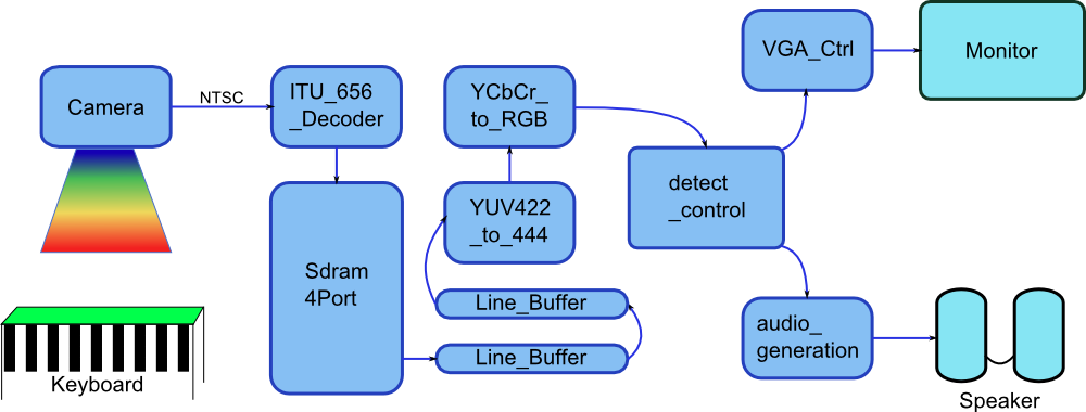
General Block Diagram
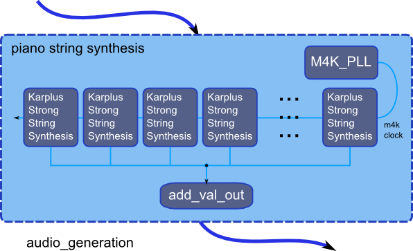
Piano sound synthesis
The development work of this project was split up into two aspects, the video signal processing and the audio signal generation. The audio signals generated were for two instruments, a drum set and a piano. The Karplus-Strong algorithm was chosen for the simulation of piano chords because of its ability to simulate the behavior of stringed instruments; in addition the algorithm is quite light weight in terms of the kinds of computations that are needed.
Karplus-Strong Background Math
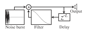
The Karplus-Strong algorithm is a method of physically modeling the behavior of string vibration, by simulating the decay of a wave on a string. It consists of a short delay line (the length of which is determined by the frequency of the note to be generated).A waveform is looped over this filtered delay line to simulate the sound of a plucked string or as in the case of a piano a hammer strike. The main components in implementing this algorithm are the delay line, the applied strike, the feedback function that determines the way the note on the string decays.
Karplus-Strong Detailed Design
The length of the delay line is determined by the intended frequency of the note being generated. The fundamental frequency (specifically, the lowest nonzero resonant frequency) of the resulting signal is the lowest frequency at which the unwrapped phase response of the delay and filter in cascade is - 2pi. The required phase delay D for a given fundamental frequency F0 is therefore calculated according to
D = Fs/F0
Where Fs is the sampling frequency. In this project 48 KHz was used as a sampling frequency F0. The rationale for choosing a high sampling frequency was that, it was found that the signals on shorter delays lines decayed faster. Selecting a higher sampling frequency allowed usage of longer delay lines with better decay characteristics. For example the delay line corresponding to the note of middle C(261.626)Hz has an approximate length of
D= 48000/261.626 => 184 entries
The actual delay line was implemented using 2 port SRAM created from M4K blocks using the Altera MegaWizard. The Karplus-Strong algorithm was implemented as a state machine, with the machine going through the following states
1) Hit- On detecting a hit, the delay line was initialized with the hit pattern which in this case was a Triangular waveform. Once the hit is complete the string starts vibrating.
2) Vibration State-During each cycle in this state, the two values at the head of the delay line are extracted, averaged and fed back to the input of the delay line with slight damping. This simulates the decay of the wave on the string. In addition the averaged output is fed to the audio DAC as an input.
3) String hold- In order to synchronize the string vibration and output generation with the Audio Clock, the delay line is only updated with new data once for every positive edge transition of the audio clock. This ensures synchronization with the Audio Clock and no samples are dropped.
Extension to multi-key system and modularizations
In order to have a greater amount of flexibility with the composition of the Karplus-Strong modules they were developed in a parameterized and modularized fashion, with each Karplus Strong module having the ability to play any given note within a range. This flexibility necessitated over-provisioning of memory for the delay line, since every module could be expected to generate the lowest possible note with a greater delay line size. Given that the system was required to support a minimum of 16 strings, this over-provisioning did not pose a problem.
Modifications to the Karplus-Strong Algorithm
The Karplus Strong algorithm is quite flexible in its ability to simulate the behavior of any stringed instrument. In order to make the algorithm simulate the behavior of specific instrument aspects of the physical design of the instrument need to be considered. For example the default Karplus-Strong Algorithm defines a low pass filtered random noise signal to be a good candidate for the initial string hit signal. The sound generated from such a waveform is similar to the pluck of a guitar with slight harshness arising out of the random string hit. Real pianos use a hammer to create the hit and the hit is thus much softer and smoother. To simulate this instead of using a random hit, the hit waveform generated was defined as an impulse/triangular waveform. The resultant audio output for such a hit is considerably smoother without the twang of a guitar.
In addition real pianos use more than one string (usually 3) strings per note, the slight difference between the lengths of the strings and the inter-string resonance due to their close proximity give the note a richer sound. In our case we were limited by the number of M4K blocks to using 2 strings to simulate each note, with the strings differing very narrowly in length. Initially the 2 strings were kept separate, with their averaged outputs feeding into the Audio output. In order to better simulate the actual behavior of a piano, the 2 strings were coupled together, with averaged output being fed back into both the strings. This led to an appreciable difference in the kinds of notes generated with the result simulating the sound of a piano to a great extent.
Once the basic piano module was working, we modified the module to play some chords. For this we predefined chords in the verilog code, where each chord needed certain keys to be played at the same time.
Performance Optimizations
Running the audio signal generation state machine and the M4K blocks at the same frequency would have meant that for every memory operation 2 cycles of delay would have been needed for the operation to complete. This would have added additional complexity to the state machine. In order to avoid this M4K blocks are overclocked and run at a clock rate of 100 MHz generated using a PLL from the 50MHz signal. Also the Karplus-Strong state machine runs at a slower rate of 27MHz, This allows sufficient time for the memory to respond from the time it receives a request, meaning that no state delays are needed and the result of the memory operation is available in the immediate next cycle from the perspective of the slower Karplus-Strong state machine.
General Block Diagram
Drum sound synthesis
The drum sound was simulated using 2D wave equation on a square mesh in order to produce the various sound effects. We used a state machine that implemented a 10x10 matrix of nodes. Due to the limitations on the availability of logic elements in the DE2 board, we used M4K block to store the node values instead of registers. This gave us flexibility to increase our drum size by duplicating the state machine modules.
Mathematical Analysis
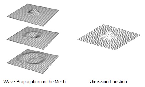
In order to create a drum-like pattern, the wave equation that we implement must give out a pattern as wave propagation on the mesh. It is evident that, given an initial excitation at some point on the digital waveguide mesh, that energy from that excitation will tend to spread out from the excitation point more and more as the traveling waves scatter through the junctions. It is not, however, easy to see that the wave propagation on the mesh converges to that on the ideal membrane. The initial excitation, i.e., the first hit closely resembles the Gaussian function as shown in the figure.
Gaussian function is given by,
for some real constants a, b, c > 0, and e ≈ 2.718281828 (Euler's number).
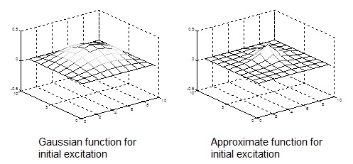
However, there is no exponential function in Verilog. So we could not directly implement this Gaussian function. We choose an approximate function that closely imitated this Gaussian function.
![]()
where amp, a, b >0 are real constants.
Below figures shows the plot of Gaussian function and this approximate function.
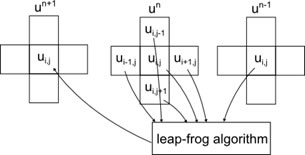
The Leap-frog algorithm with the Finite Difference model is used in order to calculate the values of each node at every time instant. This is given by,
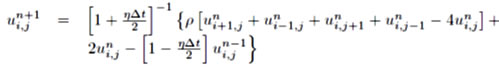
where η is the viscosity coefficient and ρ=(Δt/Δx)2. This equation is obtained by representing the 1-D wave equation in second order Taylor expansion. Below diagram explains how the above equation works on a 2D mesh.
Mathematical model hardware implementation
In order to implement this algorithm in Verilog code, we replaced the fraction by parameter ‘eta’ which decides the damping of the sound produced and used parameter ‘rho’ for ρ which decides the pitch of the sound. Each ‘ui,j’ in the equation represent a node at position (i,j) and un+1 represents the value of the node at next time instant, un represents the value of the node at current time instant and un-1 represents the value of the node at previous time instant. The values for rho and eta were selected in such a way that we did not have to use any multiplier in our code but instead use arithmetic shift operators ‘<<<’ and ‘>>>’. In a left arithmetic shift of a binary number by 1, the empty position in the least significant bit is filled with a zero. Note that arithmetic left shift may cause an overflow; this is the only way it differs from logical left shift. In a right arithmetic shift of a binary number by 1, the empty position in the most significant bit is filled with a copy of the original MSB. This is shown in the figure below. So in order to use a value of ρ as 0.125, we assigned rho to 3 and right shift the term that gets multiplied by rho by 3 bits.
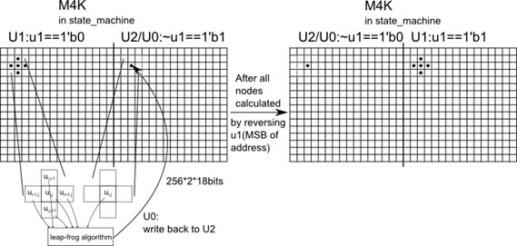 We used a single state machine that computes a 10x10 node matrix. This state machine used a M4K block to store the node values instead of registers. Now for implementing the Finite Differences wave equation, we needed four blocks of M4K memory. One to store the initial excitation values, one to store the value of the nodes at current instant (u1), one to store the value of the nodes at next instant (u) and one to store the values of the node at previous instant (u2). We removed the memory required to store the initial excitation values by calculating it each time dynamically whenever KEY3 was pressed. We also removed the memory required to store the next value (u). We instead stored the next value calculated, in the block of memory that was used to store the previous value (u2); since once a particular node from the previous instant block (u2) was used, it was no longer needed, thereby replacing that node with its next value (u). Thus from four blocks of memory we came down to just two blocks thereby reducing the size of the M4K RAM. This optimization helped in increasing the number of state machine modules.
Since we had to send out signals to the Audio Codec’s output, we were synchronizing our state machine with the Audio Codec with the help of the AUD_DACLRCK. Thus we started a computation at every positive edge of AUD_DACLRCK and if the computation finished soon then we waited for the next positive edge. We used wires x_offset, y_offset, x_boundry and y_boundry in the state machine to determine the offsets for each state machine module and the boundaries for the entire mesh. Since we are expanding our mesh in only one direction, we are hardcoding values of y_offset and y_boundry to zero. We used 10 input and output wires for each module to communicate to its neighbouring module. The state machine initially sets all the M4K blocks to value zero during reset and then checks if KEY3 is pressed. When pressed it excites each node to a certain value as decided by the approximate function and then computes the next instant node values using the leap-frog algorithm. We used switches in order to select the number of nodes in the mesh and to select the values for rho and eta.
Genral Block Diagram

Everything put together
Finally, after putting all the modules together we get our final Air Piano and Air Drum. We used two DE2 boards for the two instruments. On one board we ran the detect control and the Karplus-Strong algorithm to give us the piano sound whereas on the other board we ran the detect control and the Leap-Frog algorithm to give us the drum sound.
General Block Diagram