ECE 5760: Laboratory 2

Multiprocessor Drum Synthesis.

For this exercise, you will simulate the 2D wave equation on a square mesh in realtime to produce drum-like sounds.
This year we will add a nonlinear effect related to the instantaneous tension in the mesh.
We will also compare drum sizes that can be simulated in realtime using HPS and FPGA.

Relevant lectures from 2017 might be lectures 13 to 17.
But remember that lab 3 in 2017 is lab 2 today.

Read Study Notes on Numerical Solutions of the Wave Equation with the Finite Difference Method.
The main result you will need to simulate is equation 2.18.
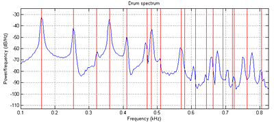
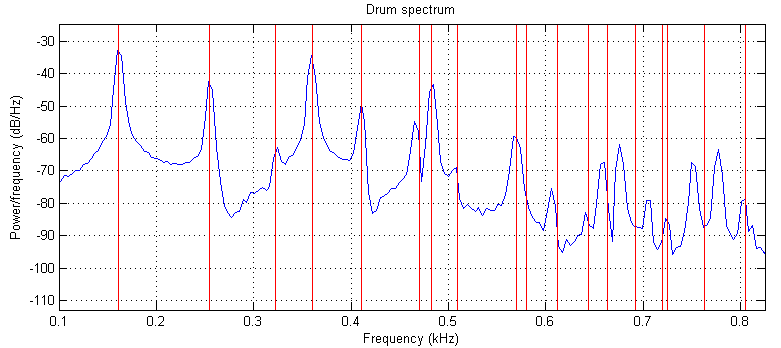
A matlab program gives a sequential version of the algorithm and plots the Fourier modes of the drum. Another version is tuned to middle C (261 Hz). You can see in the figure below that the simulated sound spectrum (blue) matches the theoretical drum modes (red) up to about mode 8 or 9 (see Physical modeling with a 2D waveguide mesh for details) . The theoretical square drum mode frequencies follow the ratio sequence:
sqrt(m+n) where m,n=1,2,3,...
Where the first term (sqrt(2)) corresponds to the fundamental mode of the drum.
The first few modes are 1, sqrt(5)/sqrt(2), 2, sqrt(10)/sqrt(2), sqrt(13)/sqrt(2), sqrt(17)/sqrt(2).

Modifying the boundary conditions, damping, wave speed, drum size, and distrubution of input energy can modifiy the sound of the simulation from drum-like, to chime-like, to gong-like or bell-like. You can modify the program further to include frequency-dependent damping and other effects. This version simluates a long, thin bar struck at one end.

Adding tension modulation allows pitch bending observed in a real drum after a large amplitude input. The large amplitude means that the membrane is stretched more, and therefore the speed of propagation (and therefore pitch) is increased. This matlab code produces an exagerated pitch effect with initial high amplitude. See also PHYSICALLY-BASED SYNTHESIS OF NONLINEAR CIRCULAR MEMBRANES equation 10.

You will probably want to read

• IMPLEMENTATION OF FINITE DIFFERENCE SCHEMES FOR THE WAVE EQUATION ON FPGA
• PARALLEL IMPLEMENTATION OF FINITE DIFFERENCE SCHEMES FOR THE PLATE EQUATION ON A FPGA-BASED MULTI-PROCESSOR ARRAY
• Time Domain Numerical Simulation for Transient Wave Equations on Reconfigurable Coprocessor Platform
• Design Methodology for Real-Time FPGA-Based Sound Synthesis

for ideas on parallelization.

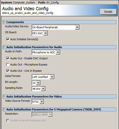
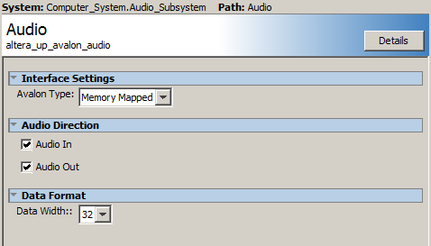
The hardware audio interface is a Wolfson WM8731 codec which is controlled by an I2C interface.

• The Qsys AVconfig module abstracts away much of the codec detail.
• The codec fast data transfer hardware is hidden behind Altera IP called the University Audio Core for Qsys (configuration interface).
• An example using the audio core is near the bottom of the Avalon Bus master page.
  

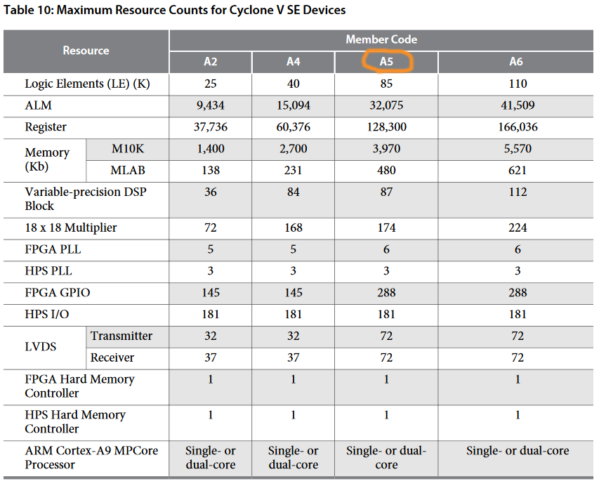
Cyclone5 handbook describing available hardware, but here is a summary.

• Also read documentation on incremental compilation. Some compile times may be very long.
• To avoid long compile read Using ModelSim to test node computations
• Generating repetitive structures:
  • Evans and Sutherland HDL guide, chapter 9, for info on using generate.
  • example shift register
  • Generate blocks from springer
  • Verilog Pro site, with some details about generation mechanism and signal scope
  • SystemVerilog Generate Construct
• Cyclone5 memory blocks.
  • Cyclone5 DSP blocks description and arithmetic megafunctions
  • HDL style -- inferring memory and DSP blocks, and a post from Mohammad

Verilog Testing:

1. Simulate one node with four zero-value boundary conditions.
   Use synthesizable Verilog running in simulation in ModelSim
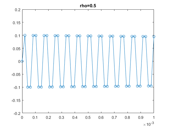
   Result should be simple harmonic motion. Remember that rho<0.5. Start with rho=1/16.
   Note that when rho is close to the limit of 0.5 that the solution has a very high natural frequency,
   so that the sine wave is on the border of aliasing, and therefore looks like a square wave.
   Assuming1:17 fixed point, start with initial conditions, uⁿ=u^n-1 and amplitude about 1/8 full scale.
   Compare to matlab solution. rho=0.5, rho=0.0625
2. Get the generate statement running and imulate the nonlinear PDE solver
   for a 24x24 (or greater) grid using no more than 174 multipliers.
   Compare to Matlab solution.
3. Get 10x10 array running using the audio codec on the FPGA for demo in second lab.
   You will want to refer to the Bus Master page, Audio output bus_master example.
   Also refer to the DSP page.
   
4. Scale up parallel processor to 40x40 or greater. Required audio output with nonlinear rho.

HPS Testing:

1. A good place to start for audio output from HPS is to search for Audio synthesis on the DSP page. The audio code example supports a finite difference drum scheme. The drum coded is a linear system with coefficients chosen so that cheap fixed-point shifts could be used to generate the 32-bit sound samples at 48Ksamples/sec. At -O3 optimization, I could just fit a 30x30 FDTD drum into the 20.8 microsecond systhesis time frame. With nonlinear rho, the maximum size was around 25x25 grid. MP3 generated by HPS on a 25x25 grid, with nonlinear rho. (wav)
   
2. Modify the code for the nonlinear rho effect. This will require rewriting the solver to use fixed point multiplies.
   
3. Get a finite difference scheme running using the audio codec on the FPGA.
   Required audio output with nonlinear rho.
4. Scale up HPS solution until it is no longer realtime.

Student examples running on FPGA:

• 2008: Matt Meister and Cathy Chen wav file.
• 2008: Parker Evans and Jordan Crittenden wav1, wav2
• 2010: Skyler Schneider wav base drum
  with n = 16 ,rho = 0.05, eta = 2e-4, alpha = 0.1, boundaryGain = 0.0, node hit = (8, 8), node probed = (8, 8)
• 2010: Peter Kung and Jsoon Kim, rho bit shifted = 6, 8, 10, 11, 14
• 2010: Kerran Flanigan, Tom Gowing, Jeff Yates, chickencan, glasshit, littlebongo, minibell
• 2011: Jinda Cui and Jiawei Yang, drum, bass drum, bowl
• 2011: Weiqing Li and Luke Ackerman, low, high
• 2011: João Diogo Falcão, growing grid, old MacDonald.
  The growing grid starts at 7*34*4=952 nodes, (#columns*#lines*symmetry), and ends at 254*34*4=34544 nodes. This is with Rho=0.5 and Eta=0.000244.
• 2014 Saisrinivasan Mohankumar, Ackerley Tng, Ankur Thakkar, eta = 0.0002, rho = 0.5 and 0.25, boundary gain =0, Number of nodes = 89x257x2 ( rows x colums x symmetry) = 45746 nodes.
  Lower, Higher
• Christine Soong, Mary had a little lamb
• Last year the highest number of nodes was around 80,000 on DE1-SoC.

Assignment

Weekly check points

1. Week 1:
   -- Simulate a 10x10 (or greater) linear grid to produce a sound by exporting the wave file to matlab.
   Use synthesizable Verilog running in simulation in ModelSim.
   -- Show the number of cycles necessary to solve the audio sample.
   -- Also demo the HPS producing a nonlinear drum sound through the FPGA audio codec.
   -- Show the time that the HPS uses to solve the audio sample.
2. Week 2:
   -- Simulate the nonlinear PDE solver for a 24x24 (or greater) grid using no more than 174 multipliers.
   Use synthesizable Verilog running in simulation in ModelSim.
   -- Use the simulation waveform to produce a sound in matlab.
   -- Demo at least a 10x10 linear solver array running using the audio codec on the FPGA
   at real-time solution rate.
   
3. Week 3: demo full FPGA system below and compare to HPS.

Full system

1. Build a realtime drum solver which produces sound from the audio codec interface.
   Minimum FPGA grid size for full credit should be at least 40x40, bigger than the size that can be solved by the HPS in realtime.
   The grid should have no more than 4:1 aspect ratio.
   Grid expansion via symmetry does not count for size.
2. The solver on the FPGA should solve the 2d wave equation to produce selectable effects.
   A minimum of three buttons on the DE1-SoC should produce different timbers.
   Timber can be set by boundary condition, eta, rho, tension modulation, or number of nodes.
   At least one timber must include audible nonlinear tension modulation effects.
3. There should be exactly one computational update of all the drum nodes for each audio sample.
   Each sample that you calculate must be output to the audio codec.
   Each node simulated will require around 10 additions/multiplications. You may be able to use clever shifting schemes to avoid multiplys. Thus the computation rate will be about
   10*(number of wave equation nodes)*(audio sample frequency) .
   For a minimal 24x24 grid you will need ~276x106 operations/sec. Clearly some parallel processing will be necessary as you go to higher numbers of nodes.
4. You can use fine-grained parallelism or course-grained multiprocessors on the FPGA side.
5. You can output sound either by using a bus-master on the FPGA, or using the HPS to feed the audio codec.
6. During the demo, prove to the TA that the computation finishes in less than 20.8 microseconds for the 40x40 or bigger drum you demo.
   
7. Record the audio output back into matlab to show that your simulation matches drum modes (under the correct boundary conditions, etc).

Be prepared to demo your design to your TA in lab.

Your written lab report should include the sections mentioned in the policy page, and :

• Mathematical considerations (what you actually implemented)
• A table of grid size versus compute time for both the FPGA solver and the HPS solver.
  Do you see any cache-size effects on HPS? What is the effect of -O0 vs -O3?
  Are there any scaling surprizes in the FPGA?
• Your parallelization scheme
• A plot of the power spectrum of your drum sounds for each different timber
• A heavily commented listing of your Verilog design (if you write a bus-master) and GCC code (if you use HPS).