Home | Introduction | My Model | Results and Discussion | References and Links
My model uses twelve neurons: ten pre-synaptic neurons and two post-synaptic neurons. It also uses two different stimuli
Stimuli: The length of each trial is 100 milliseconds. Both stimuli (numbered 1 and 2) are applied from t=40 to t=70. Most simulations were run with 100 trials, meaning that the timer was run from t=0 to t=100 exactly 100 times with the weights of the synapses adjusted after each trial and carried over to the next trial. Most simulations were also run with alternating stimuli strengths of 100 and 50. More precisely, if trials are numbered from 1 to 100, odd trials featured a stimulus 1 strength of 100 and stimulus 2 strength of 50. Even trials featured a stimulus 1 strength of 50 and stimulus 2 strength of 100. This alternation of stimuli strengths allowed stronger network recognition of both stimuli to develop over time.
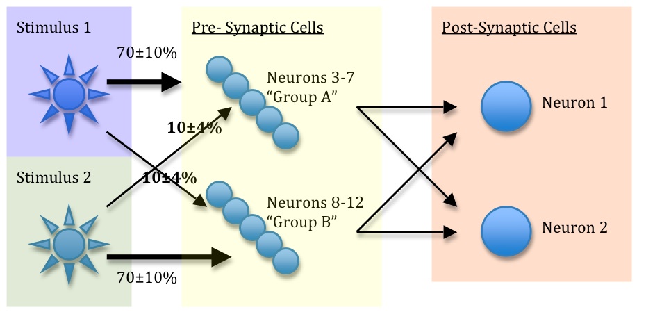
Pre-synaptic Neurons: The presynaptic neurons are numbered 3 through 12, and are further grouped into two different sets: neurons 3-7 (group A) and neurons 8-12 (group B). Group A neurons were more strongly stimulated by stimulus 1 and group B neurons were more strongly stimulated by stimulus 2. More specifically the neurons in group A received an average of 70% of the strength of the applied stimulus 1 and only an average of 10% of the strength of the applied stimulus 2. Neurons in group B received an average of 70% of the strength of the applied stimulus 2 and only an average of 10% of the strength of the applied stimulus 1.
Noise was built into the system by allowing the strength of the stimulus reaching each individual neuron to vary with every trial. Fractions of the strengths of stimuli reaching neurons were normally distributed for each neuron. For example, on any given trial, neuron 3 would receive some fraction of stimulus 1's strength with a mean of 70% and standard deviation of 10%. Neuron 3 would also receive some fraction of stimulus 2's strength with a mean of 10% and a standard deviation of 4%. Other neurons in group A were similarly stimulated in each trial. Neurons in group B had a similar stimulation profile, switching the means and standard deviations for the two stimuli. This construct is made more clear below.

Post-synaptic Neurons: The post-synaptic neurons are numbered 1 and 2. Initially, every pre-synaptic neuron (3-12) has an equal synaptic weight on each post-synaptic neuron. e.g. Neuron 3 has a synaptic weight of 0.1 (again arbitrary and relative) on neuron 1 and a synaptic weight of 0.1 on neuron 2. Neurons 4 through 12 feature the same synaptic weights on neurons 1 and 2. A matrix of the synaptic weights would look like this, where element(1,2) is the weight connecting:(neuron 1 output spike) to (neuron 2 input synapse):
SynStrength = ...
[0 0 0 0 0 0 0 0 0 0 0 0;...
0 0 0 0 0 0 0 0 0 0 0 0;...
0.1 0.1 0 0 0 0 0 0 0 0 0 0;...
0.1 0.1 0 0 0 0 0 0 0 0 0 0;...
0.1 0.1 0 0 0 0 0 0 0 0 0 0;...
0.1 0.1 0 0 0 0 0 0 0 0 0 0;...
0.1 0.1 0 0 0 0 0 0 0 0 0 0;...
0.1 0.1 0 0 0 0 0 0 0 0 0 0;...
0.1 0.1 0 0 0 0 0 0 0 0 0 0;...
0.1 0.1 0 0 0 0 0 0 0 0 0 0;...
0.1 0.1 0 0 0 0 0 0 0 0 0 0;...
0.1 0.1 0 0 0 0 0 0 0 0 0 0] ;
In such a situation with equal synapse strengths, both neurons 1 and 2 receive exactly the same amount of stimulation from neurons 3-12 regardless of the respective strengths of stimuli 1 and 2. Thus, a small modification was made in order to guide the process of self-organization. Neuron 3's synapse on neuron 1 was made stronger than neuron 3's synapse on neuron 2. Similarly, neuron 8's synapse on neuron 2 was made stronger than neuron 3's synapse on neuron 1. In this way, neurons 3 and 8 somewhat guided the rest of the neurons in groups A and B, respectively, to adjust their synapse weights. The revised matrix of synapse weights looks like this:
SynStrength = ...
[0 0 0 0 0 0 0 0 0 0 0 0;...
0 0 0 0 0 0 0 0 0 0 0 0;...
0.18 0.02 0 0 0 0 0 0 0 0 0 0;...
0.1 0.1 0 0 0 0 0 0 0 0 0 0;...
0.1 0.1 0 0 0 0 0 0 0 0 0 0;...
0.1 0.1 0 0 0 0 0 0 0 0 0 0;...
0.1 0.1 0 0 0 0 0 0 0 0 0 0;...
0.02 0.18 0 0 0 0 0 0 0 0 0 0;...
0.1 0.1 0 0 0 0 0 0 0 0 0 0;...
0.1 0.1 0 0 0 0 0 0 0 0 0 0;...
0.1 0.1 0 0 0 0 0 0 0 0 0 0;...
0.1 0.1 0 0 0 0 0 0 0 0 0 0] ;
The Learning Algorithm: The learning algorithm involved is a normalized version of the generalized hebbian algorithm, known as Oja's Rule (see the introduction section). The weight (w) connecting neuron 3's output to neuron 1 is read off the matrix shown above. The input variable (x) into neuron 1 from neuron 3 is defined as the number of times that neuron 3 fires during the stimulus period (t=40 to t=70) times the weight (w) connecting neuron 3 to neuron 1. Thus, if neuron 3 fired 10 times during the stimulus and the weight connecting it to neuron 1 was 0.1, the input variable x into 1 from 3 would be 10*0.1 = 1. The input variable from neuron 3 into neuron 2 and from neurons 4-12 into neurons 1 and 2 were similarly defined and calculated.
The output variable (y) of each neuron 1 and 2 was one of two possibilities. In the activity-independent case, y for neuron 1 was calculated by summing all of the input variables x from neurons 3-12 into neuron 1. For neuron 2, y was calculated by summing all of the input variables x from neurons 3-12 into neuron 2.
In the activity-dependent case, y for neuron 1 was calculated as simply the number of times that neuron 1 fired during the stimulus period (t=40 to t=70). Similarly, y for neuron 2 was calculated as the number of times that neuron 2 fired during the stimulus period.
Applying Oja's rule for updating the weight of synapses, the weights of each synapse were updated according to the following equation (for the pre-synaptic case). SynStrength is the matrix showing synapse strengths. LR is defined as the learning rate, and it was kept at 0.002 for most simulations. SumPerNeuron is the output varaible in the activity-independent case, calculated as described above. FiredTimesSynapse is the input variable, calculated as described above.
SynStrength(k, j)=SynStrength(k, j)+LR*SumPerNeuron(j)*(FiredTimesSynapse(k, j)-SumPerNeuron(j)*SynStrength(k, j));
In the activity-dependent case, the equation is modified as shown. The only difference is the output variable, now shown as the number of times either neuron 1 or 2 fires during the stimulus period (t=40 to t=70).
SynStrength(k, j)=SynStrength(k, j)+LR*countNumberOfFiresPerCell(j)*(FiredTimesSynapse(k, j)-countNumberOfFiresPerCell(j)*SynStrength(k, j));
One of these two equations was applied over all neurons 3-12 (k) for both neurons 1 and 2 (j).
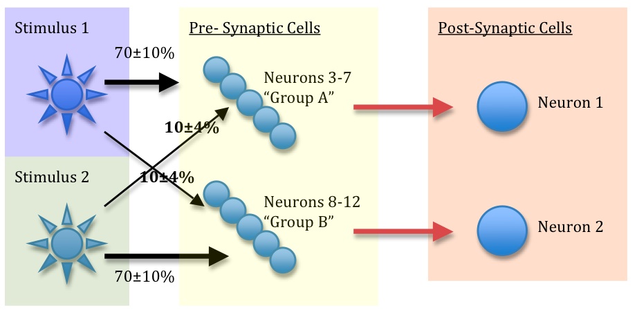
Applying this algorithm after each simulation over 100 simulations, it is observed that neurons 3-12 will adjust their synaptic weights to synapse most strongly on either neuron 1 or neuron 2, depending on which group they are in. In the case described above where neuron 3 (part of group A) begins more strongly connected to neuron 1, all of the other neurons in group A tend to become more strongly connected to neuron 1 over time and less strongly connected to neuron 2. A similar effect is seen with neuron 8 dragging group B towards neuron 2. This is illustrated in the following diagram (note the strong red arrows).
