Home | Introduction | My Model | Results and Discussion | References and Links
For a single trial, the spiking activity of all neurons is plotted below. In this particular trial, stimulus 1 has strength 100 and stimulus 2 has strength 50. Neurons in group A spike more strongly because each receives an average of 70% of stimulus 1, which is stronger. Neurons in group B spike less strongly because they only receive an average of 10% of stimulus 1, though they still receive 70% of the stimulation from stimulus 2. Notice that most of the spiking occurs during the stimulus period (t=40 to t=70).
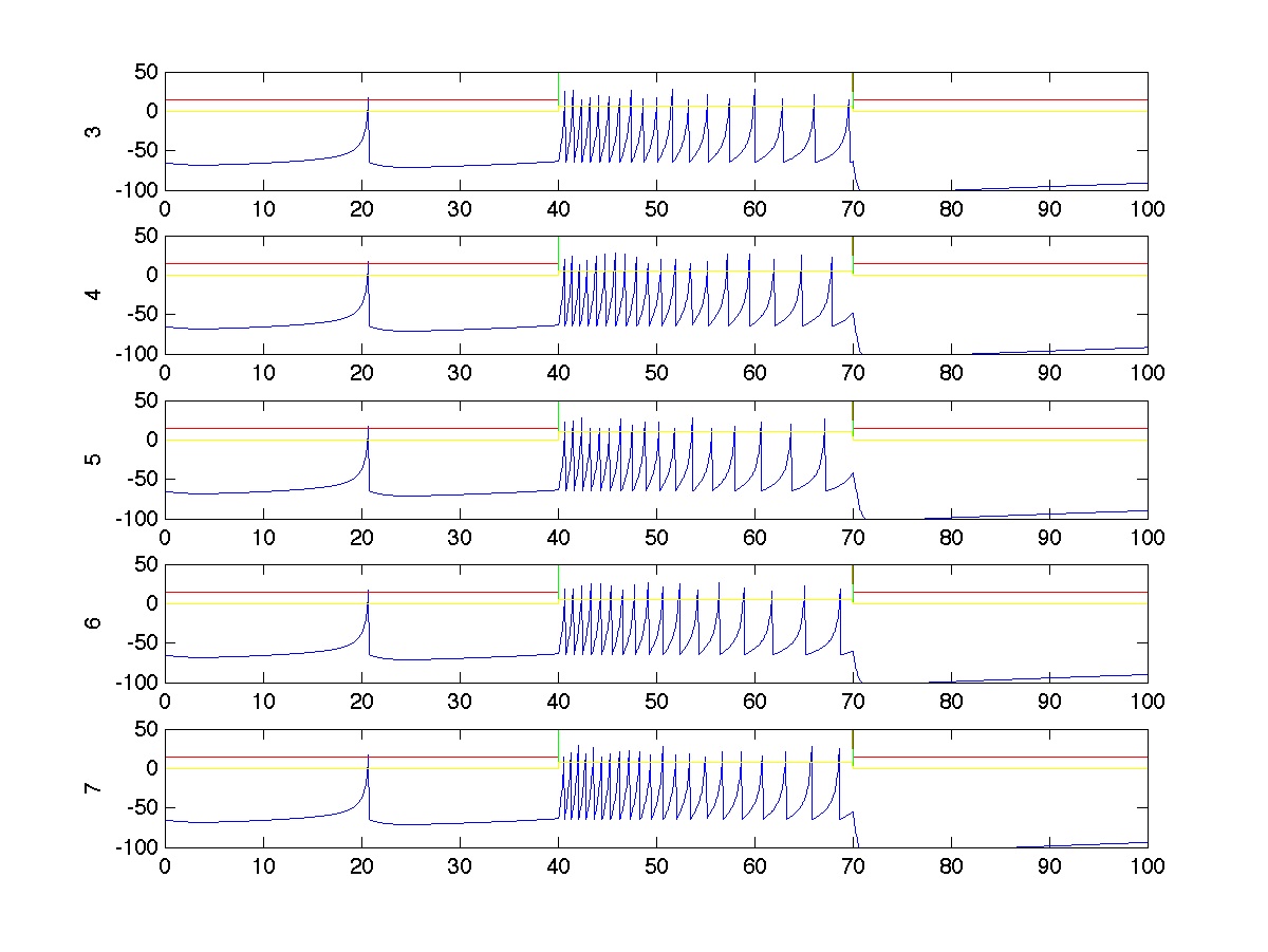
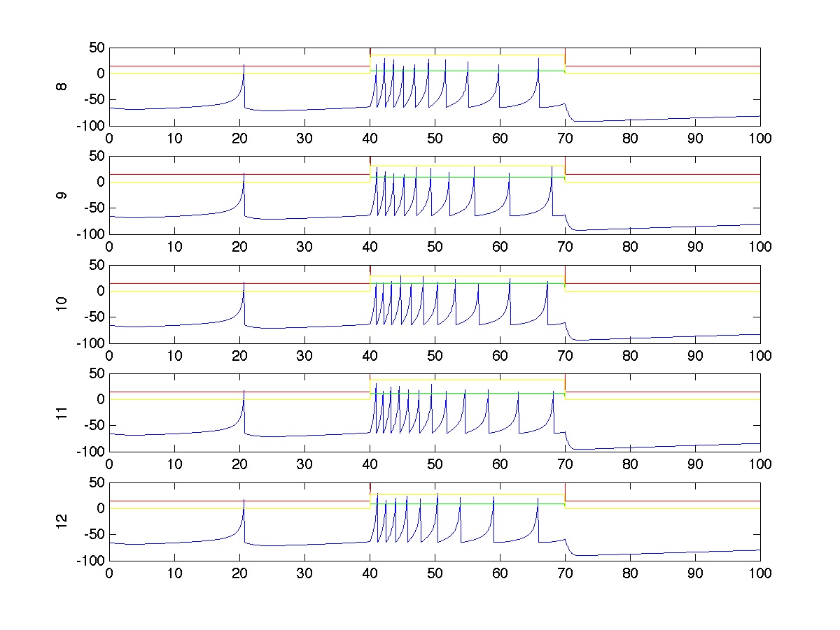
The spiking activity of the two post-synaptic neurons are also shown. In this case, neuron 1 spikes exactly one more time than neuron 2 during the stimulus period because neuron 3, which receives reacts more strongly (70%) to stimulus 1 (which is stronger than stimulus 2) synapses more strongly on neuron 1 than on neuron 2.

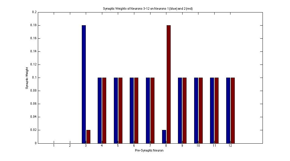
This bar graph shows the distribution of synapse weights before any Hebbian learning. Note the predisposition of neuron 3 towards neuron 1 and neuron 8 towards neuron 2.
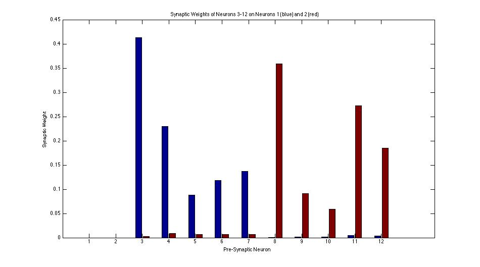
This bar graph shows the distribution of synapse weights after an example learning simulation. This learning simulation was done using Oja's Rule with a activity-independent output variable. Using Oja's Rule with a post-synaptic output variable produces similar results. Notice that neurons 3-7 have almost entirely lost their synapses on neuron 2 and neurons 8-12 have almost entirely lost their synapses on neuron 1.
Qualitatively and visually it is very obvious that the pre-synaptic neurons are self-organizing by stimulus. However, it was desired that this degree of organization be quantified in order so that using activity-independent and activity-independent variables for learning could be compared. Thus, the measure of connectivity was devised. The connectivity of neuron 1 is defined as,
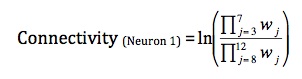
where w denotes the weight of the synapse connecting neuron j to neuron 1. The connectivity of neuron 2 is analogously defined as,

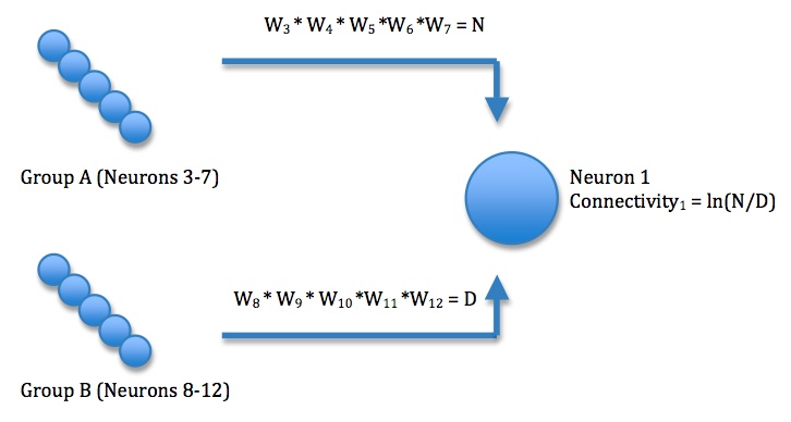
The connectivity for each of neurons 1 and 2 is increased by strengthening the synapses of pre-synaptic neurons that “should” synapse on it and weakening the strength of synapses of the pre-synaptic neurons that “should not” synapse on it. Neurons that “should” synapse on neuron 1 are those that are in the same group as the neuron that starts with a stronger synaptic weight on neuron 1. More specifically, neurons 3-7 (group A) “should” synapse more strongly on neuron 1 because neuron 3 begins with a predisposition towards neuron 1. By multiplying the synapse strengths of those neurons that “should” synapse on neuron 1 and dividing by the synapse strengths of those neurons that “should not” synapse on neuron 1, each neuron in the “should” set has equal influence on the connectivity variable, and each neuron in the “should not” set has equal influence on the connectivity variable.
The computed variable tends to increase exponentially over time. Thus, the log of this variable is taken as the connectivity because it compresses the range of values. The computation of connectivity for neuron 1 is illustrated here:
The following is a bar graph showing two different degrees of connectivity. Using the formula described above for the following network, neuron 1 is calculated to have connectivity 23.41 while neuron 2 is calculated to have connectivity 4.63

The connectivity of neuron 1 using the activity-independent output variable was computed for 50 different simulations. In addition, the connectivity of neuron 1 using the ativity-dependent output variable was also computed for 50 different simulations. The results are shown below:
Using Activity-Independent Output Variable (n=50):
Mean Connectivity = 19.663 (s.dev. = 4.938)
Using Activity-Dependent Output Variable (n=50):
Mean Connectivity = 14.5575 (s.dev. = 4.5356)
A two-sample T-test on these stats shows that the connectivity of neuron 1 using the activity-independent output algorithm is significantly greater than the connectivity of neuron 1 using the activity dependent output algorithm. (t=5.384, p= 0.000000252, df = 97.3)
Thus, using the parameters chosen for my model, it is clear than neurons are better at self-organizing if the learning algorithm relies on an activity-independent output variable rather than an activity-dependent output variable. This may help explain why post-synaptic output (in the form of a feedback circuit) is unnecessary to mediate learning in a simple Hebbian algorithm.
One issue that arose in the computation of connectivity is that occasionally, perhaps for one in ten simulations, the connectivity would be negative, which was unexpected and is still not fully understood. Further, the system is very dynamical and occasionally the synaptic weights would actually change to be negative. This was usually pretty rare and was considered to be one of the side-affects of a higher learning rate that allowed faster organization.
With more time, I would try modifying parameters such as the initial synaptic weights, the learning rate, and the stimulus strengths and see what effect there would be on the connectivity.