Cornell University
Electrical Engineering 476
Fixed Point DSP functions in GCC
using MAC in asm

Introduction

This page concentrates on DSP applicaitons of 8:8 fixed point in which there are 8 bits of integer and 8 bits of fraction stored for each number. The emphasis of these implementations is on speed, but accuracy considerations are addressed.

This page has the following sections:

• 2nd order IIR Filters
• 2nd order Butterworth low/high/bandpass filters
• 4th order Butterworth bandpass Filters
• Cascaded integrator/comb (CIC) filters
• Waveform generation (sine and white noise)
• Fast Fourier Transform
• Discrete Cosine Transform
• Fast Walsh Transform
• Karplus-Strong, FM and additive sound synthesis

Digital Filtering

One of the most demanding applications for fast arithmetic is digital flitering. Atmel application note AVR201 shows how to use the hardware multiplier to make a multiply-and-accumulate operation (MAC). The MAC is the basis for computing the sum of terms for any digital filter, such as the "Direct Form II Transposed" implementation of a difference equation shown below (from the Matlab filter description).

    a(1)*y(n) = b(1)*x(n) + b(2)*x(n-1) + ... + b(nb+1)*x(n-nb)
                          - a(2)*y(n-1) - ... - a(na+1)*y(n-na)

The y(n) term is the current filter output and x(n) is the current filter input. The a's and b's are constant coefficients, determined by some design process, such as the Matlab butter routine. Usually, a(1) is set to one, but as we shall see below, setting a(1) to a power of two may increase filter accuracy, at the cost of slightly increased execution time. The y(n-x) and x(n-x) are past outputs and inputs respectively. You can use the Matlab filter design tools to determine the a's and b's. There are also various web-applets around which help design coefficients:

• IIR filters, but note that the definitions of a's and b's are reversed and that the indexes are zero-based, rather than one-based. This applet assumes a sample frequency of 8000 Hz, but you can scale to other sample rates by making the normalized cutoff frequency, (cutoff frequency)/(Nyquist frequency)=(cutoff frequency)/4000, the same.
• Finite precision effects.

The IIR filter description is summarized in an article I wrote for Circuit Cellar magazine (manuscript).

Technical Note: To print floating point, the GCC linker options (click on [Linker options] in Project-> configure options->Custom options) must include the following specifications: -Wl,-u,vfprintf -lprintf_flt -lm. See AVRLIB description and a tutorial, but note that the tutorial has a misprint near the end. One linker option is left out in the tutorial.

Second order IIR Filters for 8:8

The 2nd order IIR code (IIRfilterGCC644.c, uart.c, uart.h, MACfix.S, zip) implements an efficient MAC operation in assembler and then uses it to produce a second order IIR filter. The time/sample is 203 cycles. It would not be reasonable to use this fixed-point algorithm with normalized cutoff frequency below about 0.10 because of the lack of relative precision in the b coefficients. With a normalized cutoff frequency=0.25, the impulse response is accurate to within 1% of peak response. With a normalized cutoff frequency=0.10, the impulse response is accurate within 5% of peak response. If you need a cutoff lower than 0.10, consider changing your hardware sample rate or using CIC filters (see below) to lower the effective sample rate. It is also possible to scale up all of the filter coefficients by 16 to give 4 bits more percision, then divide the output of the filter by 16 for each sample. IIRfilterScaledGCC644.c is an example which executes in 225 cycles. This Matlab program allows you to simulate the effect of coefficient truncation on filter response.

Another approach used in speech synthesis is to use impulse-invariant second order filters which are a bit quicker to execute because they zero out two of the general second order filter coefficients (b(2) and b(3)). These filters can also be designed on-the-fly in a C program, rather than using Matlab. It is possible to build bandpass and lowpass filters using this technique, but you need to be careful of aliasing effects and the sensitivity of coefficients to 8-bit truncation. This matlab program allows you to estimate truncation errors and design filters. Note that the bandpass filters have a gain greater than one in the passband, so you may need to scale output to avoid overflow of fixed point numbers. At 8000 Hz sample rate, you can expect to get reasonable bandpass filter accuracy down to F=250, BW=25 Hz, and lowpass accuracy down to BW=250 Hz. Impulse invariant second order filter design process:

1. Choose the bandpass center frequency, F. If the filter is to be lowpass, set F=0.
2. Choose the bandpass bandwidth, BW. If the filter is to be lowpass, the cutoff frequency is BW/2.
3. Compute: C = -exp(-2*pi*BW*T) where T=1/(sample rate)
4. Compute: B = 2 * exp(-pi*BW*T) * cos(2*pi*F*T) where T=1/(sample rate)
5. Compute: A = 1 - B - C
6. The filter output at time i is then output(i)=A*input(i) + B*output(i-1) + C*output(i-2)
7. In some circumstances generating a table of A, B and C at the frequencies you need will be the fastest way to change between filters.
   These two programs suggest how you might do this for lowpass and bandpass filters.

Second order and fourth order Butterworth IIR Filters for 8:8

If you use a Butterworth approximation for lowpass (maximally flat IIR filter) then you can simplify the general IIR filter further to only three MAC operations. Since b(1)=b(3)=0.5*b(2), the three multiplies on the first line below can be combined into one multiply by sum of inputs, with one input shifted left.

b(1)*x(n)+b(2)*x(n-1)+b(3)*x(n-2) = 
b(1)*x(n)+2*b(1)*x(n-1)+b(1)*x(n-2) =
b(1)* (x(n)+(x(n-1)<<1)+x(n-2))

b(1)*x(n)+b(2)*x(n-1)+b(3)*x(n-2) = 
b(1)*x(n)-2*b(1)*x(n-1)+b(1)*x(n-2) =
b(1)* (x(n)-(x(n-1)<<1)+x(n-2))

b(1)*x(n)+b(2)*x(n-1)+b(3)*x(n-2) = 
b(1)*x(n)+0*b(1)*x(n-1)-b(1)*x(n-2) =
b(1)* (x(n)-x(n-2))

A 4th order Butterworth bandpass filter (2 poles on lower side, 2 on upper side) can be done in 5 multiplies since b(1)=b(5)=-0.5*b(3) and b(2)=b(4)=0. Impulse response accuracy is within 2% after 10 samples with cutoffs of [0.25 0.35]. As the bandwidth of the filter gets smaller, the b coefficients get smaller also and roundoff errors get worse. Various tools exist to choose filter coefficients, for example the Matlab command [b,a]=butter(2,[Flow,Fhigh]) will generate the coefficients for this bandpass filter.

Since adding and shifting are much faster than multiplying ,we get a speedup. The 2-pole butterworth high and low pass execute in 151 cycles, the 2-pole bandpass in 148 cycles and the 4-pole butterworth bandpass in 242 cycles. All three second order filters and the fourth order bandpass are in one test program (IIRfilter2and4GCC644.c, uart.c, uart.h, MACfix.S, zip).

As before, accuracy of fixed point filters is always a concern. As the filter bandwidth gets narrower, the accuracy decreases. This is because the b(n) coefficients become smaller and roundoff/truncation error dominates. We can minimize truncation errors by scaling the filter coefficients and the filter code. As an example, if we set a(1)=16, and multiply all of the other coefficients by 16, then the value of the output does not change, but 4 more bits are available to store the scaled filter coefficients.

CIC filters

CIC filters are a form of optimized FIR filter with uniform coefficients. For example, an FIR filter with coefficients 0.2*[1 1 1 1 1], which is a 5 point running average, could be implemented using a CIC filter. For general use, CIC filters are considered crude, but they are widely used as a antialiasing prefilter before down-sampling a signal to a slower sample rate. See also Multirate Techniques and CIC Filters by Robert Lacoste, Circuit Cellar issue 231, Oct 2009, page 50ff.

This CIC filter example is a fourth order filter and 4-times downsampler. The filter attenuates frequencies above the new (lower) Nyquist frequency by about 50 db (factor of 300). The effective passband is about 0.25 of the new Nyquist frequency. A matlab test program is included as a comment in the C source code. The filter takes 170 cycles when it is only integrating, but 360 cycles when it is doing the downsampling and comb filtering. A version with better bandwidth incorporates a Chebyshev compensator to increase the passband to about 0.42 of the new Nyquist frequency. The Chebyshev filter uses ripple in the passband to compensate for droop in the CIC filter. The filter takes 180 cycles when it is integrating, 330 cycles when it is integrating and Chebyshev filtering, and 360 cycles when it is doing the downsampling and comb filtering. You could interleave other IIR filter operations into the remaining filter phases. Another version of the fourth order filter only downsamples by a factor of 2, but keeps the Chebyshev compensator for good bandwidth.

This CIC filter is a second order filter and 4-times downsampler. The filter attenuates frequencies above the new (lower) Nyquist frequency by about 25 db (factor of 17). The effective passband is about 0.4 of the new Nyquist frequency. The filter takes 100 cycles when it is only integrating, but 190 cycles when it is doing the downsampling and comb filtering. Significant aliasing can occur with this filter, but it may be good enough for some applications where speed is more important that quality.

Waveform Generation

Sine wave synthesis by direct digital synthesis (DDS) and noise synthesis by 31-bit linear feedback shift register are demoed in this program. The sample rate is 62,500 samples/sec, which is the highest PWM rate at 16 MHz clock rate.

Fast Fourier Transform (FFT) for 8:8

I adapted the int_fft.c program from this webpage. I simplified the program for real-only input and forward direction only (no inverse FFT). The function returns the real and imaginary components of the transform. The table gives the exectuion times in cycles and mSec (at 16 MHz clock) as well as the time to accumulate the input samples at 8 kHz. At an 8 kHz ADC sample rate, the FFT runs faster than real time up to 128 samples (FFT time < Sample time). In an actual spectrum estimation application, you would need to add time for windowing the input and combining the real and imaginary outputs (sums of squares or sums of absolute values) to get the power or amplitude.

Code is FFTfixGCC644.c, multASM.S, uart.c, uart.h, project zip.

There are many uses for a FFT including filtering, convolution, and pattern matching. Some applets.

Discrete Cosine Transform (DCT) for 8:8

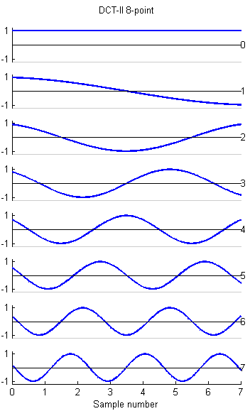
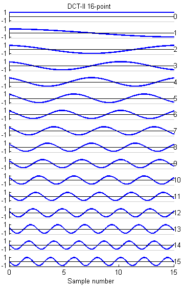
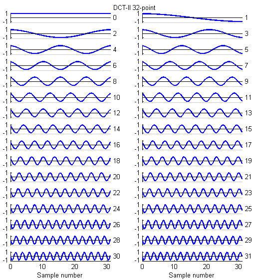
The DCT is a variant of the FFT which is used in image, sound, speech, and video processing and compression. I wrote 8,16 and 32-point versions based on the code in a web page by Yann Guidon <whygee@f-cpu.org> shows an optimized verion of the DCT-II algorithm for 8 points. I modified the code for GCC and assembler. The 16-point version was derived by combining two 8-point transforms. The book by KR Rao and P Yip Discrete Cosine Transform: Algorithms, Advantages, Applications (Academic Press 1990, pages 60-61) show how to combine transforms. The 32-point version was derived by combining two 16-point transforms. The test program requires multASM.S, uart.c and uart.h.

The 32 point DCT-II runs in 4640 cycles, or about 0.29 millseconds with a 16 MHz clock. This is fast enough to do some real time speech spectral analysis. At a sample rate of 8 KHz, a 32-point transform would cover 4 mSec of samples. Since the first (non-DC) harmonic is 1/2 cycle in a 4 mSec window, the fundamental of the transform is 125 Hz (low enough to catch a male voice fundamental) and the maximum frequency is about 3400 Hz (high enough to catch most information for speech). A matlab program which shows the spectral analysis properties of the DCT is here.

The basis functions for the 8, 16 and 32-point versions shown below are similar to the FFT, but capture gradients with fewer coefficients. For example, the first basis function (not the zeroth) in all images encodes an almost linear gradient, something which takes a sum of several basis functions of a Fourier series. The Matlab program to generate the plots is here.

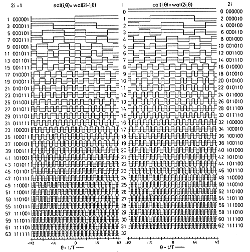
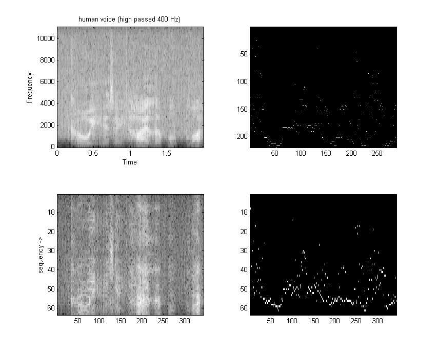
Fast Walsh Transform (FWT) for 8:8

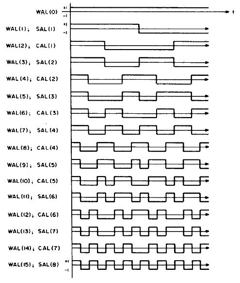
I wrote a FWT which converts a time sequence to coeffieients of the orthogonal Walsh-function basis. An example of the first 16 basis functions from Jacoby and 64 basis functions from Pichler is shown below. Odd functions are called sal, analogous to sine, while even functions are called cal. The following functions are in arranged in sequency order. Sequency is defined as the number of zero crossings, and is anaogous to arranging sines in frequency order.

1. The first algorithm I used was from Manz. It was first converted to Matlab code, then to C. The Matlab code compares the FFT and FWT outputs as spectrograms, then takes the maximum of each time sliced transform and compares these spectrograms. Examples are spectrogrms for a chirped sine, chirped square wave, a woodthrush, and a fragment of human speech. FFT power spectrum is the top row, FWT sequency spectrum (sum of absolute value of sal and cal coefficients) is the bottom row. Both transforms are 128 points. The right column of images has been formed from the left by finding the maximum intensity coefficient of each spectrogram time slice. Note that the max component of the FFT and FWT match fairly well. Jacoby has useful information on using FWT. Ritter has a good biblography. This C program executes a 16 point transform in 2120 cycles (with optimization set to Os). the program requires uart.c and uart.h. Note that the output of the FWTfix routine is not in sequency order (it is actually in dyadic order). Order is not important for some applications. Run the FWTreorder routine to make a sequency order, but note that you must use the correct length reorder array. The reorder routine takes about 780 cycles to order 16 points.
2. Removing the normalization from the FWT inner loop drops the execution time to 1995 cycles, but can cause overflow if longer transform lengths are used or if the average data approaches full scale for 8:8 numbers.
3. The second algorithm I used was from from Hugh Larson, An algorithm to compute the sequency-ordered FWT, IEEE Transactions on Acoustics, Speech and Signals, Aug 1976 page 335. This program version is hard-coded for 16-points, is unnormalized, and executes in 595 cycles. Including the conversion to sequency order, it is over 4 times faster than the general version above.
4. This C program attempts to light up leds corresponding to which sequency bands have the most energy. The program takes a 16 point FWT at a sample rate of 7.8 kHz, throws away the DC component, adds the absolute value of the sal and cal components, then lights an LED if the component is the maximum and above a threshold. It requires an analog input on A.0 and LEDs attached to PORTC.

Sound Synthesis

Karplus-Strong Algorithm, digital waveguides

The Karplus-Strong Algorithm (KSA) for plucked string synthesis is a special case of the digital waveguide technique for musical instrument synthesis. The KSA is particularly well suited for implementation on a microcontroller, and was originally programmed on an Intel 8080! The simplest version hardly needs fixed point arithmetic, but better approximations do require some more sophisticated digital filters. The basic algorithm fills a circular buffer (delay line) with white noise, then lowpass filters the shifted output of the buffer and adds it back into itself. The length of the buffer (along with an allpass fractional tuning filter and the sample rate) determine the fundamental of the simulated string. The type of lowpass filter in the feedback determines the timber. Prefiltering the white noise before loading the buffer changes the pluck transient timber. A matlab program to generate a plucked string is here. The equivalent C code is here. The C code takes about 10% of the cpu (at a 8000 Hz sample rate) to generate one string.

Driving the Karplus-Strong string with a synthesized waveform expands the range of sounds you can make. In this version of the program, the string can be plucked using an initial waveform consisting of noise, sawtooth, triangle or sine wave. It can also be driven by an exponentially rising and falling waveform of all the previous types. A matlab program was used for testing, then converted to a DDS plus KSA C code. In the C code, each sample takes, around 420-500 cycles to compute. The PWM output is filtered through a simple RC lowpass with a cutoff of 10,000 radians/sec (about 1600 Hz). The string length of 61 (at 8000 Hz sample rate) corresponds to approximately note C3 (130.8 Hz). The examples below are generated from the C code.

Changing the loop lowpass filter to a one-pole butterworth with a normalized cutoff of 0.2 (800 Hz), putting a one-pole butterworth highpass with a cutoff of 0.2 in the output, and introducing some clipping makes a sound which is vaguely clarinet-like. The matlab code. The C code and an example. The C code executes in about 440 cycles/sample at 8000 Hz sample rate.

Changing one plus to a minus makes a brassy percussion sound with a duration determined by the length of the delay line. More information can be found in referneces below.A generalization of the digital waveguide technique involves multiple waveguides, each with a bandpass filter. This is refered to as banded waveguides and is explained in papers by Essl, et.al (see below). The aim of banded waveguide programs is simulate spectrally complicated drum, bar (e.g. vibraphone), or multiple-string instruments. A matlab program to compute one banded waveguide is here. A banded waveguide with several diferent buffer lengths, and hence natural frequencies, (but no interaction between modes) is here. Modifying the program for additive mode interaction changes the sound somewhat. Parameters to control include: ratios of the different circular buffer lengths, width of the bandpass filters for each buffer, value of the damping factors for each buffer, and weights of the additive mixing. Please note that many of these techniques are patented by Stanford University and licensed to Yamaha and others.

ECE4760 projects which have used KSA

• 2007 air guitar (video 23MB mp4 ).
• 2008 air drums
• 2008 dualing banjos

FM synthesis

An alternative to Karplus-Strong physical synthesis is to use FM modulation of a sine wave to approximate the sound of various instruments. Two matlab programs (1, 2) produce various string-like, chime-like or bell-like tones, depending on the FM parameters. A single FM modulator C version for Mega644 executes in about 220 cycles/sample, or about 10% cpu load at a 8000 Hz sample rate. There are several example parameter sets at the end of the C code. Two FM modulations (C program) applied to one DDS takes about 280-340 cycles/sample. Both of these programs could easily run at 16000 samples/second for better bandwidth. A third C version includes wave tables for different modulation shapes. The following table is from the third C version.

Additive synthesis

Additive synthesis attempts to match the Fourier spectrum of the desired sound. A matlab program and C program add three harmonics. The C program takes about 450 cycles/sample. At 8 KHz sample rate this is about 20% of the cpu time. Adding a high quality noise generator to the additive synthesis bumps up execution time to 970 cycles, but can make a steel drum effect. Adding three wavetable options (sine, sawtooth, and triangle) and reducing the quality of the random noise generator takes execution time to around 600 cycles/sample.

For the matlab program, with 5 additive frequencies, the following parameters and sounds give some idea of the capabilities of additive synthesis:

clarinet-like
f1 = 262 ;
f2 = 262 *2 ;
f3 = 262 * 3 ;
f4 = 262 * 4 ;
f5 = 262 * 5 ;amp1 = 1; fall_time1 = .7 ; attack_time1 = 0.7 ;
amp2 = .05; fall_time2 = .7 ; attack_time2 = 0.7 ;
amp3 = .5; fall_time3 = .7 ; attack_time3 = 0.7;
amp4 = 0.01; fall_time4 = .7 ; attack_time4 = 0.7 ;
amp5 = .2; fall_time5 = .7 ; attack_time5 = 0.7 ;

plucked string
f1 = 262 ;
f2 = 262 *2 ;
f3 = 262 * 3 ;
f4 = 262 * 4 ;
f5 = 262 * 5 ;
amp1 = 1; fall_time1 = .7 ; attack_time1 = 0.01 ;
amp2 = 1; fall_time2 = .3 ; attack_time2 = 0.01 ;
amp3 = .5; fall_time3 = .1 ; attack_time3 = 0.01;
amp4 = .3; fall_time4 = .1 ; attack_time4 = 0.01 ;
amp5 = .1; fall_time5 = .1 ; attack_time5 = 0.01 ;

drum
f1 = 262 ;
f2 = 262 * 1.58 ;
f3 = 262 * 3 ;
f4 = 262 * 2.24 ;
f5 = 262 * 2.55;
amp1 = 1; fall_time1 = .7 ; attack_time1 = 0.01 ;
amp2 = 1; fall_time2 = .3 ; attack_time2 = 0.01 ;
amp3 = 1; fall_time3 = .1 ; attack_time3 = 0.01;
amp4 = .3; fall_time4 = .4 ; attack_time4 = 0.01 ;
amp5 = .3; fall_time5 = .1 ; attack_time5 = 0.01 ;

bell
f = 523*2.
f1 = f ;
f2 = f * 1.58 ;
f3 = f * 3 ;
f4 = f * 2.24 ;
f5 = f * 2.55;
amp1 = 1; fall_time1 = .7 ; attack_time1 = 0.01 ;
amp2 = 1; fall_time2 = .3 ; attack_time2 = 0.01 ;
amp3 = 1; fall_time3 = .1 ; attack_time3 = 0.01;
amp4 = .3; fall_time4 = .2 ; attack_time4 = 0.01 ;
amp5 = .3; fall_time5 = .1 ; attack_time5 = 0.01 ;

References

• A Tutorial on Digital Sound Synthesis Techniques, Giovanni de Poli,: Computer Music Journal, Vol. 7, No. 4 (Winter, 1983), pp. 8-26
• Physical modeling using digital waveguides
  Julius O. Smith, III
  Computer Music Journal, Vol. 16, No. 4. (Winter, 1992), pp. 74-91.
• Digital Synthesis of Plucked-String and Drum Timbres
  Kevin Karplus; Alex Strong
  Computer Music Journal, Vol. 7, No. 2. (Summer, 1983), pp. 43-55.
• Extensions of the Karplus-Strong Plucked-String Algorithm,
  David A. Jaffe; Julius O. Smith
  Computer Music Journal, Vol. 7, No. 2. (Summer, 1983), pp. 56-69.
• Theory of Banded Waveguides
  Essl, Georg, Serafin, Stefania, Cook, Perry R.,Smith, Julius O. (Julius Orion)
  Computer Music Journal, Volume 28, Number 1, Spring 2004
• Musical Applications of Banded Waveguides
  Essl, Georg, Serafin, Stefania, Cook, Perry R.,Smith, Julius O. (Julius Orion)
  Computer Music Journal, Volume 28, Number 1, Spring 2004
• A review of musical synthesis techniques from 2006 is Discrete-time modelling of musical instruments, by Valimaki V, Pakarinen J, Erkut C, Karjalainen M, in REPORTS ON PROGRESS IN PHYSICS 69 (1): 1-78 JAN 2006
• http://web.eecs.utk.edu/~qi/ece505/project/proj1.pdf
• http://www.eee.hku.hk/~ugsnews/lab-sheet/level2/lab04.pdf.
• https://ccrma.stanford.edu/~sdill/220A-project/drums.html#fm
• The Synthesis of Complex Audio Spectra by Means of Frequency Modulation

The codevision/Mega32 DSP page has older versions.

Copyright Cornell University April 12, 2011