Home

Introduction

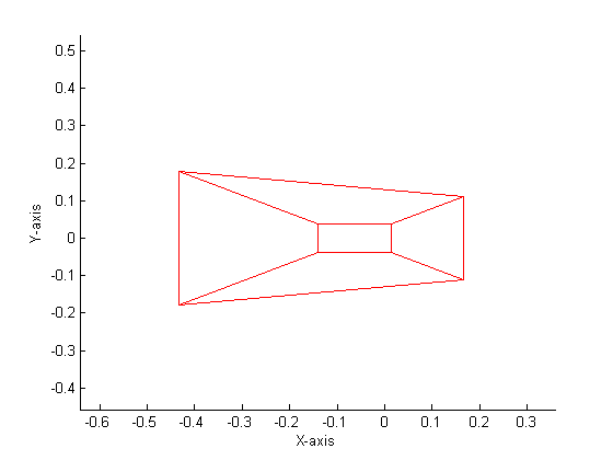
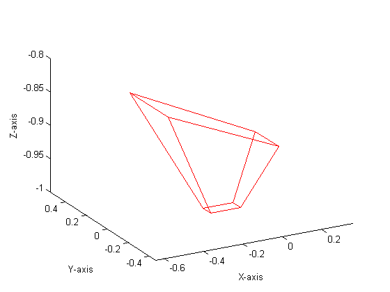
Software Design

Hardware Design

Results

Issues

Conclusion

More Pictures

Here is our top level microcontroller C code.

Our ultimate goal in software was to have a programmer only specify the vertices of triangular polygons in any space they desire, a camera position, and a camera angle, and have supporting software perform the rest of the calculations.

Because of the complexity of perspective transformations, it was necessary to do a first run-through in Matlab. Here, we tested our designs for algorithms that would later be devectorized and ported into C.

There are two main steps that need to be performed before calculating a perspective transformation: the conversion from world space to view space, and then from view space into canonical space. World space is what the coordinates are originally given in. View space uses the camera vector and angle to tilt and distort world space appropriately. The conversion between the two can be accomplished via a matrix transformation. View space is then transformed into canonical space, which uses preset variables to define a coordinate system in {-1 < x < 1, -1 < y < 1, -1 < z < 1} in which all viewable points lie. Points outside this box in canonical space represent lines outside the field of vision.

Three vectors are needed in order to start this process. The vector e is the camera point in world space. This becomes the origin in view space, since everything is viewed from the camera’s perspective. The vector g defines the gaze direction: a vector from e that indicates where the viewer is looking. Finally, the vector up, which defines the up direction: in our case, this is [0, 0, 1] since up is always in the +z direction.

From these vectors, we are able to calculate and scale u, v, and w, which become the orthonormal basis of view space. u = up × w v = w × u w = -g

We can now define the matrix that we need in order to move from world space to view space, which ends up being simply a rotational transformation followed by a translation.

When performing these calculations, it also makes it easier computationally to be able to scale without any recriminations. Hence, each coordinate is converted from three-space into four-space:

Each four-dimensional homogeneous coordinate has only one corresponding point in three-space, and has the property that scaling the vector does not change its real representation.

To move from view to canonical space, we need to define a set of variables based on what we want to actually be inside of our view space. The four things that need to be defined are the field of view in X and Y, the near plane, and the far plane. The field of view is straight forward: the value in degrees that defines how far you can see in X and Y. Since, in window view, Y = 0.75X, we related the FOVs of X and Y. We used an X of 150º and a Y of 112.5º. The near and far planes (n and f, respectively) are used to clip what we are viewing in the Z direction. The closer you can place n and f together, the easier it is to perform computation.

From these values, we are able to create a transformation matrix to scale view space into canonical space:

where M_wc = M_vcM_wv.

Once in canonical view, the next step is to clip the polygon appropriately. For this, we chose the Sutherland-Hodgman algorithm because of its simplicity and effectiveness. It only works with convex polygons, but this is a restriction of our system to begin with, so it was no big change. Sutherland-Hodgman, as we implemented it, works like this:

For each clipping edge

For each edge of the polygon with endpoints <i, j>

Check whether <i, j> are inside the polygon:

(Yes, Yes): append node j to the list

(Yes, No): calculate where the edge hits the clipping wall and append the clipped point to the list

(No, No): add nothing to the list

(No, Yes): calculate where the edge hits the clipping wall and append both the clipped point and j to the list

Next

Reset the list of edges to those just calculated

Next

This algorithm is able to clip a polygon of n-sides into canonincal space. Naturally, our clipping edges were X = ±1, Y = ±1, Z = ±1. By limiting our input polgons to three-sided triangles (which gives us the added advantage of not accepting nonplanar surfaces), polygons that this clipping algorithm outputs can have 0, 3, 4, 5, or 6 edges, depending on what is clipped.

By applying these algorithms in Matlab, we were able to produce a mathematical perspective projection.

Our Matlab code is included here.

Some outputs are shown below.

What the viewer would see on the screen: the graphic mapped to the X-Y plane.

How the hardware sees the image: the 3-D planar image underlying the visual output.

Our conversion of this Matlab code first required us to devectorize the matrices. After doing (and re-doing and re-doing) these out by hand, these were the basic formulas we came out with:

where c₁, c₂, c₃, and c₄ are predetermined constants, e•u, e•v, and e•w are calculated once earlier in the code in order to streamline the process, and c is the homogeneous scaling factor. Using these formulas, we are able to reduce our amount of floating point multiplies to 12 per vertex.

Near the end of our project, it became clear that depending on where the viewer was facing, a polygon could be sent counter-clockwise with respect to the screen and viewer. Thus, we needed a way to sort the polygon in a clockwise fashion with respect to our mirrored Cartesian coordinate system.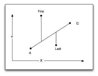

The methodology we use is wonderfully simple: we find the upper-leftmost point A, and then compare it to its two neighbors, B and C. If C lies above the line of A and B in our mirrored VGA screen coordinate system, the points must be sent with A being first and B being last. If C lies below the line of A and B, the points of the polygon must be sent with A being first and C being last.