Cornell University Cornell ECE 1 ECE 5760

• Hardware Design
• DE2 Module
• SRAM Controller
• Initialize Module
• Fractal and Cascade Land
• Gaussian
• Orthographic
• Erase
• Rotator
• RandomMod
• Color Scheme
• Keys and Switches

Hardware Design

The physical hardware used for this project consists of an Altera DE2 FPGA board, an external VGA monitor and a connecting VGA cable. The rest of the hardware design is implemented using verilog, which is run by downloading it to the FPGA. For more, see Appendix B.

The following figure shows the structure of our hardware design and the communication links between the several modules in our design.

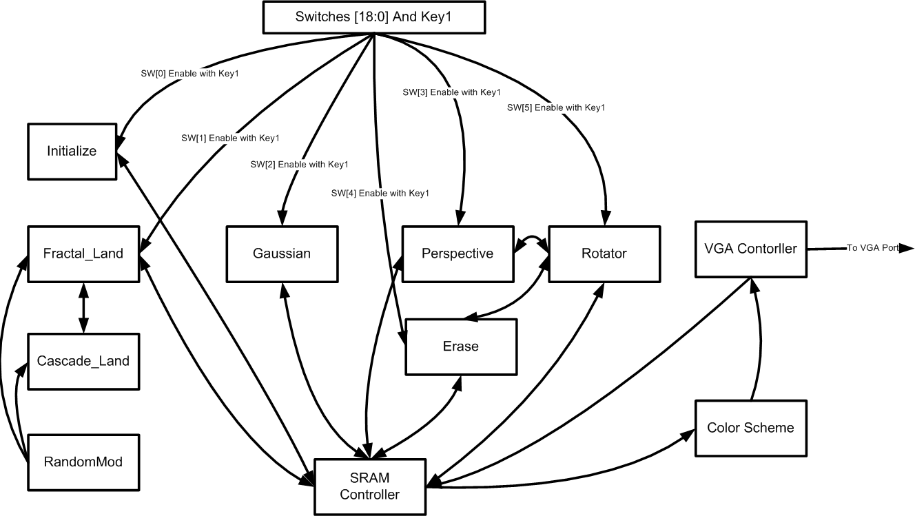
Figure1: Top Level Block Diagram

 

DE2 Module

The DE2_Default was our top level verilog module and it was mainly used to instantiate the various hardware modules used in the design and define communication busses between them. All of the modules described in this section have an enable signal and a kick-start signal. The enable signal is used to select a particular module for execution and the kick-start signal resets the module and starts its execution again. The following is a discussion of some of the key hardware modules.

 

SRAM Controller

This module was responsible for handling the reads and writes of all other modules to the SRAM. Our entire design is clocked at a frequency of 50.4 MHz and this clock is used to generate a VGA clock frequency of 25.2 MHz that is outputted to the external monitor. Due to the writing and reading constraints posed by the bandwidth of the SRAM interface, only one read or write was allowed during a VGA clock cycle but different priorities were assigned based on the kind of data being read of written to the SRAM. The iState input to the controller is used to decide whether a read or write is requested to the SRAM. Whenever the VGA_SYNC control signal is high in the top module, the VGA controller wants to read from the SRAM and thus, priority is given to a VGA read in the SRAM controller by setting the iState signal to 0 externally and all other modules are stalled in the design. As soon as the VGA_SYNC signal goes low, iState signal is set to the read (0) or write (1) based on the Write Enable signals coming from the module currently executing in the system.

To handle reads, the SRAM controller takes in the full 19 bits of the address and correctly formats it such that address sent to the SRAM is of 18 bits. Since the resolution of our screen is 640x480, every 16 bit data value represents 2 pixels on the screen. Thus, only 8 bits are assigned to each pixel. Handling writes to the SRAM is a bit tricky as the 8 bit input data need to be correctly positioned in the 16 bit data value based on the input address. Thus at the positive edge of the VGA clock (OR positive edge of system clock), data is read from the SRAM based on the address provided for the write. Within 1 system clock cycle, it is expected that correct data will be read from the SRAM. Thus on the next positive edge of the system clock (when the VGA clock is 0), the data that was read is parsed and the input data (to be written) is positioned at the correct byte and fed back to the SRAM. This is how writes are handled within one VGA clock cycle. Since VGA syncs and reads are handled by the SRAM controller, all the other modules in the system never bother with the VGA addresses and data and do not keep track of them.

 

Initialize Module

This module is used to erase the entire screen and initialize the boundaries around the fractal landscapes as well as the 4 corners required to compute the landscape. It simply runs an X and Y counter that traverse from one edge of the screen to the other and based on the ranges observed, a specific value is written to the SRAM (create a boundary, erase the screen or initialize the points). This module is only executed once after resetting the entire system.

 

Fractal Land and Cascade Land

 This module is the most integral and the most important module of our design and required the most time to implement. A combination of these 2 modules implements the algorithm described in the High Level Design section and the following description discusses the implementation of this algorithm using only registers!!

Firstly, one must understand the complexity of this problem and the issues that can be faced by implementing a recursive algorithm in hardware. The fractal landscape was chosen to be contained in a 257x257 pixel grid and based on the algorithm, each point has to be uniquely calculated using the 4 similar points in neighboring squares. The algorithm starts from 1 square during initialization and at every iteration, it generates 4 more squares for every square existing on the grid and it recursively descends into each square to effectively calculate all the points on the landscape. Hence, by the end of 8th iteration, we are basically keeping track of 48 or 65536 squares. Each square is represented by the top left pixel position and bottom right pixel position. Each pixel needs to be represented by 18 bits at least (if we’re making our design on the left side of the screen). This totals to around 295KB!! Stating the obvious, this is impossible to store in SRAM and this is a very naïve approach to computing the fractal as it is just brute force implementation and doesn’t consider any optimizations at all. It is possible to store this in SDRAM but this algorithm has a lot of memory accesses and since data transfer from SDRAM is much slower compared to SRAM, it would have slowed down the entire computation for the landscape.

Our design is able to compute a landscape in real-time using a cascaded computation approach and only uses the SRAM and an array of registers to compute all the pixels in the landscape! The following sections describe how the algorithm was implemented and the various optimizations that we were able to implement given time restrictions.

First, I will describe a few basic concepts required to understand the algorithm implementation. As illustrated by the algorithm in the High Level Design, each point in the grid is a height representation or the z coordinate of that point. The value of the height is later used by the ColorScheme module to compute a color gradient for that point. Thus, the SRAM is used to store a height map of the 257x257 landscape. A RAM_256 module is used for storing all the square points generated by the algorithm. This module essentially contains 256 registers of 36 bits, which is used for storing 2 18bit pixel addresses in each register ‘line’. Each line can thus contain a single square representation on the screen by storing the pixel addresses. The Fractal_Land as well as the Cascade_Land modules consist of 2 of these RAM modules (each). The usage of these is described as follows. The Fractal_Land module is used to compute the first 4 iterations of the algorithm and the cascade land is used to the last 4 iterations.

The data calculation part of the algorithm, for computing the pixel values, is described as follows. In every iteration, for every square that is fetched from the RAM, the 4 data values corresponding to the 4 corners of the square are fetched from the SRAM and a diamond step is run to calculate the center point of the square. Subsequently, for the square step of the algorithm, 9 points (4 corner points, 1 center point of current square and the 4 centers of neighboring squares) are fetched from the SRAM and calculations for the square step are run to compute the values of the of the centers of the edges of the square. In each of these steps, a random number is added to the point (as defined by the algorithm) to introduce randomness in the terrain. This randomness is successively decreased in every iteration so that there is not much variation at higher iterations and we get a smoother terrain gradient. These 2 steps have to be computed for every square alternately. To better explain this, the diamond step is executed first on all the squares present on the landscape and then, the square step is executed on all the squares. This is not the same as computing the diamond step and square step for one square and then going to the next square (this is wrong). If we individually computed the steps for each square, it would lead to discontinuity in the landscape and would give a very blocky appearance. Hence, the diamond step is executed first on all existing squares and only then do we compute the square step for all squares. After computing these 2 steps, we descend to the next iteration where we have current number of squares x4. The states required for computing the 2 steps are essentially fixed as it always requires you to perform a certain number of memory accesses to read and write the points into SRAM and thus, not much optimization could be performed for this part of the algorithm.

However, a lot of optimization can be performed for storing the square pixels at each step. This section discusses the address calculation part of the algorithm, which computes the address of each square required for the next iteration.  At the onset of the algorithm, the Fractal_Land module is fed with a single square that represents the top left and bottom right corners of the entire landscape boundary. This square line is stored at the first position in the RAM0 (assume the 2 RAMs are RAM0 and RAM1). During computation of the square and square steps, addresses are computed for the center and edges of the square for storing the calculated data values. These same addresses can be used for generating the 4 squares required for the next iteration of that square.  Hence using the first square line in RAM0, 4 new square lines are calculated and stored in RAM1. Since there was only 1 line in RAM0, the counter reaches its limit and the RAMs are switched for the next iteration. Now, the lines in RAM1 are read during the 2nd iteration and the 4 new square lines generated for each line in RAM1, are store in RAM0. Thus, by the end of the 2nd iteration (after computing all the 4 square line in RAM1), we have 16 new square lines in RAM0. The RAMs are switched again such that in iteration 3, we read from RAM0 and write to RAM1. Thus, at every iteration in Fractal_Land, we alternate the functionality of the RAMs such that we are reading from one RAM and writing to the other. Thus, one RAM is essentially used as SWAP space. Consequently, by the end of the 4th iteration, we will have 256 square lines in RAM0. This ends the main computation part of the Fractal_Land module for the first 4 iterations.

Now, the Fractal_Land module controls the functionality of the Cascade_Land module. Cascade_Land differs in functionality from the Fractal_Land module mainly in address/ square corner calculations. The data computation, the square and square steps, essentially remain the same. From earlier description, recall that we need to compute the diamond step for all squares before computing the square step. For the Cascade_Land module, assume we are using 2 more RAM modules (RAM2 and RAM3). For the 5th iteration, for each square line present in RAM0 in Fractal_Land, we initialize the Cascade_Land with that a single square line in RAM2 and let the module compute the diamond step. We again, initialize the Cascade_Land module with the next line from RAM0 and let it compute the diamond step. This is done for all the lines in RAM0. A similar procedure is used to compute the square step for all the lines in the RAM0. Now to go to the 6th iteration, we need 1024 squares (256 x 4). How do we compute this? All the data in RAMs 2 and 3 is wiped, whenever we initialize it with a new square line.

To compute the 6th iteration, we initialize Cascade_Land with a single square line from RAM0 and inform it that we need squares for the next iteration. Thus, Cascade_Land will compute the next 4 squares before performing the diamond step. Thus for the 6th iteration, every time Cascade_Land is initialized with a new square line, it will compute the next 4 squares in RAM3 and use the lines from RAM3 to compute the diamond step. After executing the diamond step for all the squares present in RAM0, the square step is computed by traversing through all lines of RAM0 again and initializing Cascade_Land at every line. In this case as well, the module will first compute the 4 squares in RAM3 that are required for the 6th iteration and then compute the square step. Similarly for the 7th iteration, for each square line added from RAM0 to RAM2 in Cascade_Land, 16 new squares are computed before performing the diamond step and square step.

This is very compute intensive as for each square line and each iteration, the Cascade_Land module has to compute all the squares required for that iteration. But this does not require a lot of cycles as the addresses can be computed very fast and we’re only interfacing with registers and not memory (which can be very slow). Hence, this algorithm proves to be very fast in computation and is able to generate a random fractal in well under 1 second!! At the end of algorithm execution, all 257x257 points are computed in the landscape (with some process noise), giving a very good gradient between mountains, plains and lakes. The following diagram tries to illustrate this algorithm sequence (for obvious reasons, the diagram cannot completely describe the entire algorithm; it only takes a stab at explaining it) and the figure following is an example output observed after execution.

 

Figure 2: RAM usage in Fractal Land Module

 

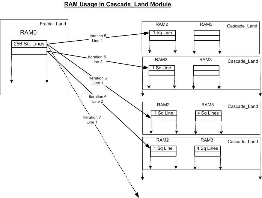
Figure 3: RAM usage illustration in Cascade Land Module

 

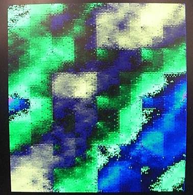
Figure 4: Raw terrain outputted after algorithm execution

Gaussian

After generating the fractal landscape using the above module, we observe that there are still tiny specks of noise in our image even though the top level structure of the landscape looks randomized (has a terrain). To smooth out the high frequency noise in our landscape (“tectonic activity??”), a 3x3 Gaussian kernel was used to convolve with the entire landscape.  Due to space and time limitations, the convolution used previously calculated pixels as well to give a successively cascaded output. This resulted in more smoothing of the landscape, even though there is tremendous loss of data with this operation. The following is the Gaussian kernel that was used:

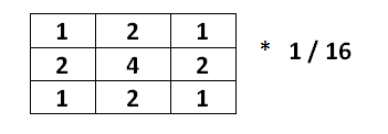
Figure 5: Gaussian Kernel used for blurring
 
The implementation of this module was very simplistic as well. X and Y counters were used to go from one corner of the landscape to the other. To calculate each pixel, 9 pixels were read from the SRAM and the kernel shown above was multiplied to the 9 pixels and the results were added together to give the intensity of a single pixel. This intensity was then stored at the address of the center pixel in SRAM and the counters were subsequently updated to the next pixel in the row.  The following is an example image after smoothing the landscape.

Figure 6: Landscape after Gaussian blurring

 

Orthographic

Once we have our smoothed image, we want to show that our landscape actually produces a good 3D representation as we hoped. This module is responsible for performing an orthographic projection by rotation the landscape around the x axis. The derivation of the formula used in the projection calculation is shown in the High Level Design.  Thus, we only have to perform calculation on the y coordinate of each pixel in the landscape using the height value present at each position pixel.

Using the above description, the implementation of this module was very simplistic as well. X and Y counters were used to go from the top left pixel of the landscape to the bottom right pixel. At each pixel, a new y value was calculated using the formula mention and it required the use of 2 multiplies and 1 subtraction. Sine and cosine ROM tables were used to look up the angles and change from one angel to the other. This ensured that the top row of the image was printed first and the last row of the image was printed last so that landscape features that were close to the eyes of the viewer overlapped the features behind it. To interpolate between various height changes, zero hold interpolation was used for 5 rows (this basically means that color is extended down by 5 rows).

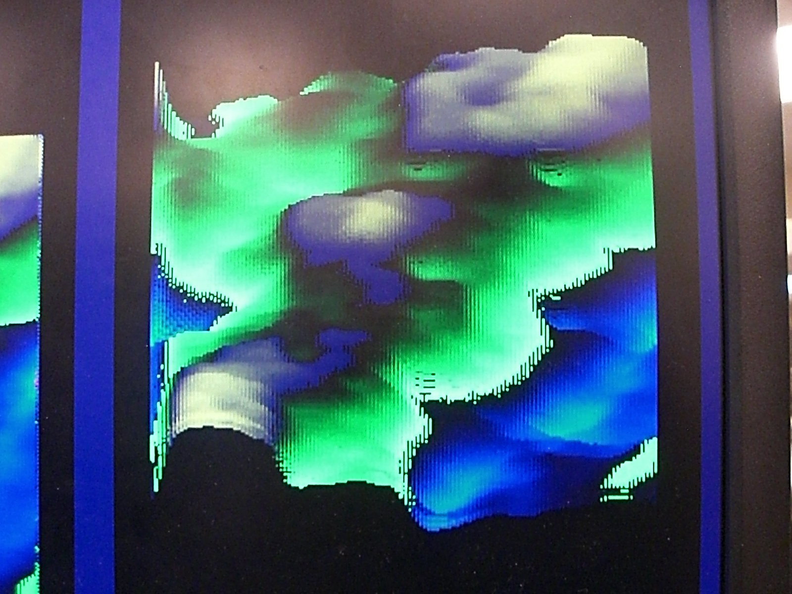
Figure 7: Landscape after rotating by 45 degrees

Erase

This module is only responsible for erasing the part of the screen where the projected image is drawn. This can be used by the user to erase the previous image and draw a new image at a new angle. This module is also used by the Rotator Module to erase after every angle change.

Rotator

This module was responsible for rotating the projected landscape image through each angle stored in the ROM (0 to 90 degrees) after certain time intervals. The state machine implemented in this module controls the Orthographic and Erase modules and draws the projected image at each angle. It first uses the erase module to erase an existing projected image. It then draws the landscape at a new angle and waits for a certain amount of time before starting over (erase -> project -> wait -> erase  . . . ). This module will keep on rotating the plane as long the enable signal is high.

RandomMod

This module is responsible for generating a random number at every VGA clock cycle. It uses a 32 bit number (which is initialized to a certain value at reset) and XORs the 31st and 28th bit and puts the result at bit0 after left shifting the number by 1 bit. This ensures the randomness of the output.

Color Scheme

This module was responsible for assigning color to the screen based on the 8 bit VGA data value read from the SRAM. Each value present in the SRAM is a height representation of the pixel and this module uses that information to assign an RGB value to the pixel. A concept similar to HSV was used to assign color as a gradient at each height and to go from one color representation to the other. Since color had to be customized for this specific project, the entire 360 variation of the HSV concept was not used, rather, a linear gradient variation was used to assign color from the lowest depth to the highest peak. The following image gives the color description according to the heights observed in the landscape:

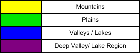
Figure 8: Color Scheme used to define regions in the landscape

 

Keys and Switches Used

The following tables list some of the keys and switches used to control the execution of each module in the design: