|
|
|
|
||
|
|
ECE5760 Final Project Adaptive Noise Cancellation Theory Highlight |
|
||
|
|
||||
|
|
||||
|
|
|
|
|
|
|
|
||
|
|
|
|
|
|
||
|
|
|
|
|
|
|
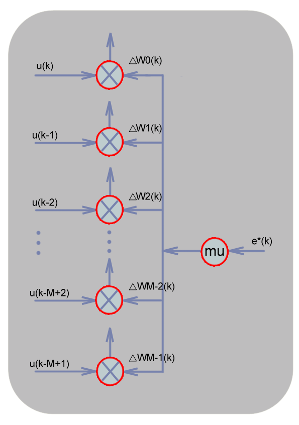
Figure.3 Details of adaptation procedure block
1. Least Mean Square Algorithm
Figure.1 Block diagram of LMS adaptive filter Figure.2 Details of adjustable filter block
2. Fast LMS Algorithm on an Adaptive Noise
Canceller
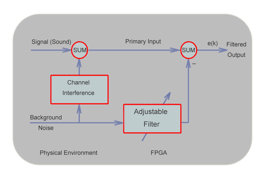
Figure.4 Structure of the adaptive noise canceller
This project is based on the least-mean-square algorithm. It was first
proposed by Widrom and Hoff at Stanford University in 1960. One significant
feature of the LMS algorithm is its simplicity. It does not require exact
measurements of gradient vector which is required by steepest-descent algorithm
and is usually not possible to compute, nor does it require matrix inversion.
LMS algorithm is simple in implementation and thus has gained tremedous
popularity in a variety of fields raning from telecommunications systems to
machine tool control to intelligent robots to audio signal processing. In this
project, an adaptive filter of 8-32 weights is implemented in DE2's FPGA and
several noise cancelling schemes are performed to verify the performance of the
adaptive noise canceller.
Figure 4 in the left is the structure of an adaptive nosie canceller. It is
a very similar to the block diagram shown in Figure 1, except that the
desired output of the adaptive noise canceller is the error signal (e=y-d)
The basic structure of the least-mean-square algorithm is shown in Figure 1,
Figure 2 and Figure 3, and can be written in the form of three basic relations
as follows:However, in order to reduce the number of multiplications of the LMS filter, a fast LMS algorithm will be used for this project so that we will have less occupancy of the logic elements which in turn will allow us to design an adaptive filter with more possible weights. The fast weight update expression is as follow: Wk+1=Wk+e(k)*sign(uk)>>>n The fast LMS algorithm uses shift operation to replace the stepsize where n is the number of shifts. Also this algorithm uses the sign bit of the reference input u(k) instead of its value. In this way the number of multiplications is significantly reduced, which will make the implementation of the LMS filter even simpler. The drawback is that learning performance will go down because of the inaccuracy caused by this simplification.
1. Filter output: y(k)=uTW 2. Estimated error: e(k)=d(k)-y(k) 3. Weights update: Wk+1=Wk+2*mu*e(k)*uk where T is the transpose operation As shown in Figure 1, the adaptive filter is supplied with the desired response d(k) and the input vector u(k) for filtering processing. The filter shown in Figure 2 produces an estimate of the desired response y(k). The formed difference between y(k) and d(k) is defined the estimation error, which alongside the input vector u(n) are applied to the feedback adjustment structure shown in Figure 3. The stepsize delta or mu in the feedback loop is inversely proportional to the settling time constant of the convergence behavior. Small values of mu will make the adaptive process slow but will largely minimize the excessive mean-square error. A large mu will make the filter converge fast, but tends to increase the excessive mean-square error (the difference between the final value J and minimum value Jmin obtained from Wiener's optimum solution)
|
|
|
|
|
|
©2011 The School of Electrical and Computer Engineering, Cornell
University
|
|
|
|
|