|
|
|
|
||
|
|
ECE5760 Final Project Adaptive Noise Cancellation FPGA Implementation |
|
||
|
|
||||
|
|
||||
|
|
|
|
|
|
|
|
||
|
|
|
|
|
|
||
|
|
|
|
|
|
|
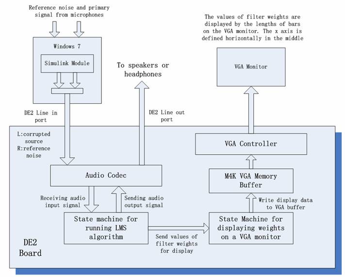
The detailed structure of the adaptive noise canceller is shown in Figure 1. In
order to perform blind filtering, the adaptive filter requires the measurements
of the reference noise and the primary input signal, which is the desired source
signal contaminated with the noise. The noise can be effectively used as the
reference only if it is measured in a field where the source is relatively weak.
Therefore, the microphone that records the reference noise must stay a certain
distance away from the one that records the primary input. The two speakers that
play the noise must be the same set so that the noise is sychronized everywhere
in the measuring field. Since a typical desktop usually has only one mic input,
two audio-to-mic USB adaptors are used to receive both the reference noise and
the primary input synchronously. For real time data acquisition and adaptive
filtering, the inputs are recorded, concatenated and played back as a stereo
output signal, which then serves as the input to the FPGA. This structure also
allows asynchronous adaptive filtering, which means that the input data can be
recorded, stored in MATLAB workspace, and used as the input to FPGA for adaptive
filtering later. In addition, a VGA monitor is used to display the values of
adaptive filter weights so that we will be able to watch the convergence
behavior of the adaptive noise canceller.
Figure 5: Weight display scheme
The state machine that implements the filter weights display is
shown in Figure 4. The weights are displayed in terms of its
magnitude and sign bit. The state machine starts with the
initialization of an iterator (the walker). The state machine will
check the current x axis coordinate of the iterator and decide which
weight this point belongs to. Once the weight target is determined,
the state machine will then check the sign bit of the weight and
negate the weight if sign(w)==1. Next the state machine will check
the current y axis coordinate and if the iterator is in the
predefined weight range the state machine writes one to the M4K
buffer at the current address. Otherwise, the state machine writes
zero to the M4K buffer. In the end, the state machine updates the
iterator and enters the next cycle. Figure 5 is the visual
illustration of the weight display scheme.
|
|
|
|
|
|
©2011 The School of Electrical and Computer Engineering, Cornell
University
|
|
|
|
|