Microcontroller Design
The microcontroller, ATMEGA32, performs a very simple task in our project; take in a reference value sent in from the serial port and run a Single-Input-Single-Output controller with distance feedback from optical shaft encoders attached to the motor.  The output of the controller is fed into a PWM module, to control the speed of the motors via an H-bridge circuit.

Motion Control
While the microcontroller’s task is simple, it is not trivial.  The control loop must work almost flawlessly, otherwise the larger, ball tracking control loop will be unstable, or unreliable.  The microcontroller must implement a feedback control loop to operate the motors, and run interrupt-driven serial communication and shaft encoder processing routines.

Electronic Hardware
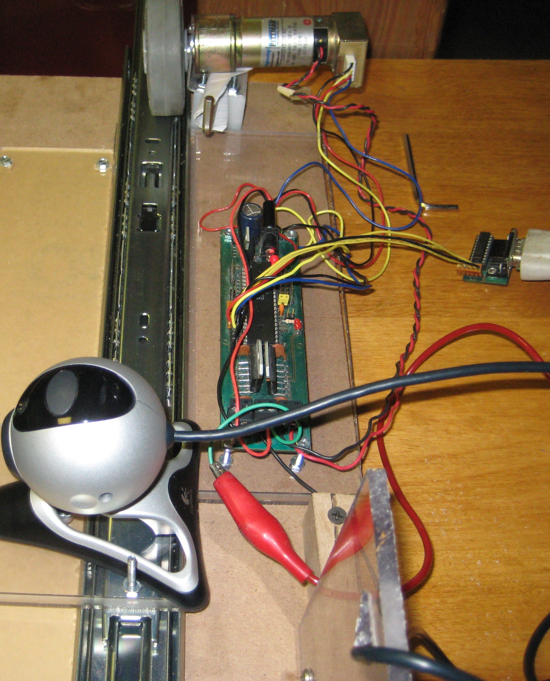
The hardware involved with the low-level motion control is a

• A microcontroller (ATMEGA32)
• A motor with shaft-encoder feedback
• A high source current power supply
• A motor control (H-Bridge) IC (LMD18200)
• A serial level converter (Max233)

Specifications
The control loop must run at a fixed frequency, so we must queue input, or reference values, as they come in.  If the control loop doesn’t run at a fixed frequency, the response of the system will change, as we are simulating a continuous system in a discrete, or sampled, fashion.
Baud rate is set to 230400 bps, for the fastest, while still reliable, data transfer rate.

Interrupts from the main control loop from the serial port and from updating the distance variable from the shaft encoder pulses must not significantly alter the main control loop’s operating frequency.

Feedback Controller Design and Specs
The specifications of the controller are:

• Zero steady state error
• All closed-loop poles are real, meaning that there are no damped oscillations in the output of the system.  All closed loop poles must lie on the negative real axis.
• Robust to slightly uneven response along track length, due to physical setup
• Reliable, i.e. little drift, over time

We decided to use a simple PI controller because it is both fast, robust when used with stable open-loop poles, and produces a zero steady-state error.  The system before feedback control is stable, or, in other words, the open loop poles of the system are stable. A proportional controller would meet spec, and performs very well, with a quick response time, Tr­.  As a matter of fact, our first approach was to simply increase K, the proportional control constant, until the steady state error was close enough to zero and the response was quick enough.
 
However, several problems arise from this approach.  Firstly, there is a time delay, partially from the time it takes to compute the sensor output, and partially from the inertia of the motor and the system.  This time delay, when used with a proportional controller with high gain K, will produce complex poles as K increases, and these complex poles will slowly, as K increases even more, wander into the unstable territory (Closed loop poles in the RHP).   To solve this problem, we chose a K­p such that the closed loop poles of the system were real, i.e full damping, no damped oscillations, but were marginally real.

We then added integral control to drive the steady state error of the system to zero.  We chose a KI, integration constant, to be much smaller than Kp so that it didn’t affect the response by driving the closed loop poles to be complex (damped oscillations in the output), but still large enough to compensate for steady state error.  We also implemented an integral wind-up checker, so that the integral would not build up too large and overflow in the microcontroller.

Our final expression for the controller is K(s)= Kp + Ki / s . Or in a proper-fraction format: K(s) = (Kp*s+Ki) / s .  The controller, however, must be brought into the discrete domain, which is very straightforward for the simple PI controller we chose.  If we chose a more complicated controller, one would have to use matlab to make a straightforward conversion from the continous s-domain into a discrete time domain.
 
K(errori)= Kp*error +Ki * SUM(errorj, j=0 to i-1).  The sum approximates the integral.  The dt time step from the integral is rolled up into the K­I constant.

The experimentally determined constants, Ki = 0.00001 and Kp = 0.06 with a feedback loop frequency of Fclk /1024 where Fclk= 14.7456 MHz.  So, Loop Freq.  = 14.4 kHz , which is more than quick enough to update changes in inputs.  The shaft encoder will output pulses around 2 kHz max.

Physical Construction
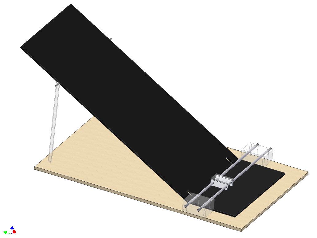
The physical layout is as shown below.  Drawings and modeling was done in Autodesk Inventor.


Materials Used:

• 2’x3’ MDF (Fiberboard)
• Clear Polycarbonate plastic
• Delron blocks
• 3/8” Aluminum rods
• Acrylic Matte-finished

The original plan, shown above, included a pully-driven cart operating on aluminum guide rails.  We revised these plans, as shown below, to use a sliding, ball-bearing, track.  The ball is placed at the top of the ramp, and rolls down the ramp where it is caught, or tracked, by the cart.   Attached are more detailed plans, including dimensions, of the final project.

Background (Black Matte-Finished Acrylic):
The background, also the ramp, is a sheet of black acrylic.  The color and finish were chosen to make the problem of object detection simpler.  However, the costly piece of plastic turned out to be far less helpful that previously imagined.  We chose to use a black ramp so that the white ball would stand out significantly, and we could implement a simple thresholding algorithm to detect the bright ball. Unfortunately, shadows and uneven lighting made this approach unfeasible, so our choice of a black background made the problem only slightly easier.  The matte finish was intended to attenuate reflections.  However, what we found was the matte finish simply blurred reflections.  So, rather than seeing reflections, there would be bright spots, or dark spots, on the background.  Again, the matte finish was an improvement, but not enough of one to significantly simply the tracking algorithm.  A painted piece of wood would have worked equally as well, and would have saved us a significant amount of money.