Computer Vision based Ball Catcher

Capturing:
To capture the video we use a Logitech webcam. The resolution is 320 x 240 pixels RGB color image. Our client program is written in Java, and employs the Java Media Framework (JMF). In this program we connect to the webcam input stream to pipe in the video and create a media player to process capture each frame as it comes in. Once a frame is captured it is sent to be processed and filtered.

Ball Detection:
In order to detect the ball we must go through a multi-stage process. The general idea in the process is to convert the image to grayscale, determine the region of interest (ROI), canny edge detect, and then perform a circular Hough transform.

The first step is to convert the image to grayscale. When we get the initial image is of 0-255 RGB value in an array of size 320 x 240. To convert, we loop through this array and perform an RGB to grayscale conversion with the following code:

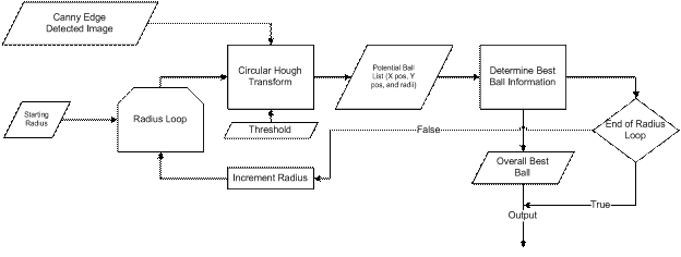
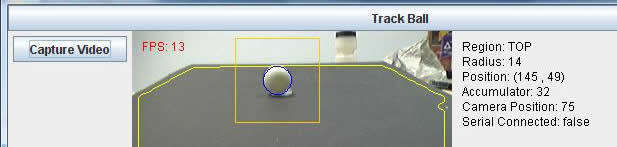
After we have converted the image to grayscale, the next thing we want to do is define the region of interest. In our setup we want the region of interest to be everything that pertains to the black sheet. Due to variations in lighting, the fact that surrounding bodies may have colors of the same as the sheet, and other issues, determining the black sheet is not as easy as a simple black thresholding. In order to calculate the region of interest, we first have to make a few assumptions. One assumption is that what the camera is currently looking at should be dominated by the black sheet, and that at the bottom of the cameras view we will always see the black sheet.

To account for the lighting in any given situation we take five regions in the image. They are centered in the top, bottom, left, right, and center of the image. Each region is 7 x 7 pixels big, and the average values of these pixels are computed. We then take the highest and lowest average values and throw them out. Out of the three remaining regions, we take the average of their values. This value is what we believe to be representative of the black colored sheet in any lighting.

After we have the hypothesized average pixel value of the black sheet we then compute the Sobel operator in both the X and Y directions to compute the gradients of the gray scale image. Next, using assumption number two that the bottom center of the camera will always be in the black region we implement a recursive function that starts at this point and searches for other similar intensity pixels and marks them as the black sheet or not. The way this works is that it moves to the right checking to see if the pixel value is within a percentage of the average and that the X and Y gradients are less than a possible edge value (because we don’t want to continue off the edge of the sheet or into the ball). Once it cannot go right, it searches up, then left, and then down. The recursive search effectively marks the entire black sheet as the black sheet, with very little error. However, to account for some error, and to compute the polygon region of interest, we have to perform the following steps. The algorithm then starts in the bottom left of the image, and moves to the right, until it finds the third marked pixel as a sheet and adds that to its edge list. Then it moves up until the top of the image. Once it reaches the top it performs the same steps, but not starting from the left side and moving to the left until it reaches its third marked pixels to set as an edge for the polygon. After this is all complete, we have defined what we believe to be the black sheet.

The next step in finding the ball is to perform edge detection on the image. Our method of edge detection is a Canny edge detector. This edge detector works by first convolving the image with a Gaussian slight blurring filter. This helps to remove noise from the image that could give false edges, while preserving dominant edge structure. Next, it calculates the X and Y gradients using the Sobel gradient operators. After this, a gradient magnitude is computed at each point. If the magnitude is greater than a threshold in which we are certain is an edge, it is marked as an edge, and if the magnitude is less than a certain threshold, it is marked as not an edge. For the middle regions, we look in the local region of the pixel to see if it is the greatest for its given direction, and if it is locally the highest, we then mark it as an edge. The end result is an array with two values, one indicating an edge, the other not an edge.

We use a circular Hough transform (CHT) to find the ball in our image. The inputs to the CHT is the Canny edge detector array, a radius value, a threshold, and a region of interest.


A CHT works by going to each pixel marked as an edge and it then traces a circle with the specified radius, centered at that edge. We have another accumulator array that has its array index incremented by one, every time a circle intersects that point. So, if you have a perfectly edge detected image, with a circle of radius R, and you input this to the CHT, you will find that at the center of that circle the accumulator value will be a maximum, because the Hough circles of radius R have interested many times over while being drawn. What we do to find these maximums is to split the image up into 16 x 16 grids and mark all pixels with highest value as a regional max. We then take the regional max pixels and check to see if their accumulator value is greater than the threshold. If it is, we record this point, along with its accumulator value, as a possible circle that could be the ball. The point list, along with the value list is returned at the end of the CHT.

We perform the CHT in a loop where the value of the radius increases from a lower bound to an upper bound, depending on where we believe the ball to be in the image. During each loop we keep track of the highest accumulator value, and its corresponding x and y values and radius. At the end of the loop we have a radius and an X and Y value that is with highest probability a circle in the desired image.

At this point we have determined where in the current image the ball lies and with what radius, assuming a ball is in the region of interest. The next step is the output to the microcontroller a position to move to so that we can catch the ball.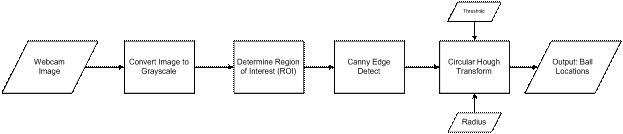

Figure: Shows the general processing steps for a given image, with wanted radius and threshold.

Figure: Shows the basic idea behind how the CHT determines which ball, if any, is the ball we want.

Speed Enhancements:
If we were to perform the ROI calculation, then the Canny edge detection on the entire image, then the CHT on the entire image, the result would be a frame rate of between 2-4 per second. This is not an acceptable value for our real time calculations. Therefore we developed a few techniques to speed up the processing.

First we had to determine what was taking the longest time in our processing. Test benches showed that the Canny edge detector was taking a lot of time to process. There were a few things wrong with how were using the edge detector. First, it was taking as an input an image, and then taking the pixels out of the image into an array. This was unnecessary, because when we determine our ROI, we have created the pixel array. Therefore, we changed the code to just pass in grayscale pixel array. Also, on each iteration, the edge detector was recalculating its kernels. Calculating the kernels only needs to be done on instantiation of the edge detector. Changing this removed unnecessary looping in the code. Also being done, is that it was outputting a binary image as its result, as opposed to a binary array.

Those were enhancements that we made directly to the edge detector, but at the time we were still operating on the entire image at a time and we thought there must be a smarter way. The smarter way we determined was to use the knowledge of previous calculations that produced an X and Y and radius location for the input image. The general idea of our state machine was that if no ball is found, we input the entire 320 x 240 image until a ball is found. When a ball is found, we then check to see what it’s Y location is. If it is in the upper third of the image, on our next iteration we will only Canny edge detect on the top half of the image, thus reducing the number of pixels to operate on in half. If it is in the middle third, we will operate on the middle half of the image (1/4 to 3/4 of the height), and if it is in the bottom third, we will input the bottom half of the input image. We also attempt to input a compressed image by a factor of two (half width and half height) after finding a ball in the ALL region. By separating the images into regions based on where the ball was previously, we were able to get rid of unnecessary edge calculations.

The next limiting factor in our processing is our circular Hough transform. What we had been doing is computing the CHT on the entire input image result from the Canny edge detector, but this was slow. To speed things up, we decided to employ another regional technique. If we had a previous value for the ball’s center and radius, we would make the input to the CHT a rectangular region that has a minimum X and Y of the previous center X and Y minus three times the previous radius, and a maximum X and Y of the previous center X and Y plus three times the radius. This we would box in the previous ball location with a guess of where the ball should be now. If it turns out our guess is wrong, on our next loop we expand the box to encompass the entire input region.

These techniques were much needed and increased our speed significantly. A table of the speed tests is included below. CED stands for Canny Edge Detector (can be fast or normal version). Fast Hough Regional is where we narrow down based on radius. Overall (bolded) you can see that the speed up was approximately 4 times, but we still lose approximately 20 FPS due to processing.