
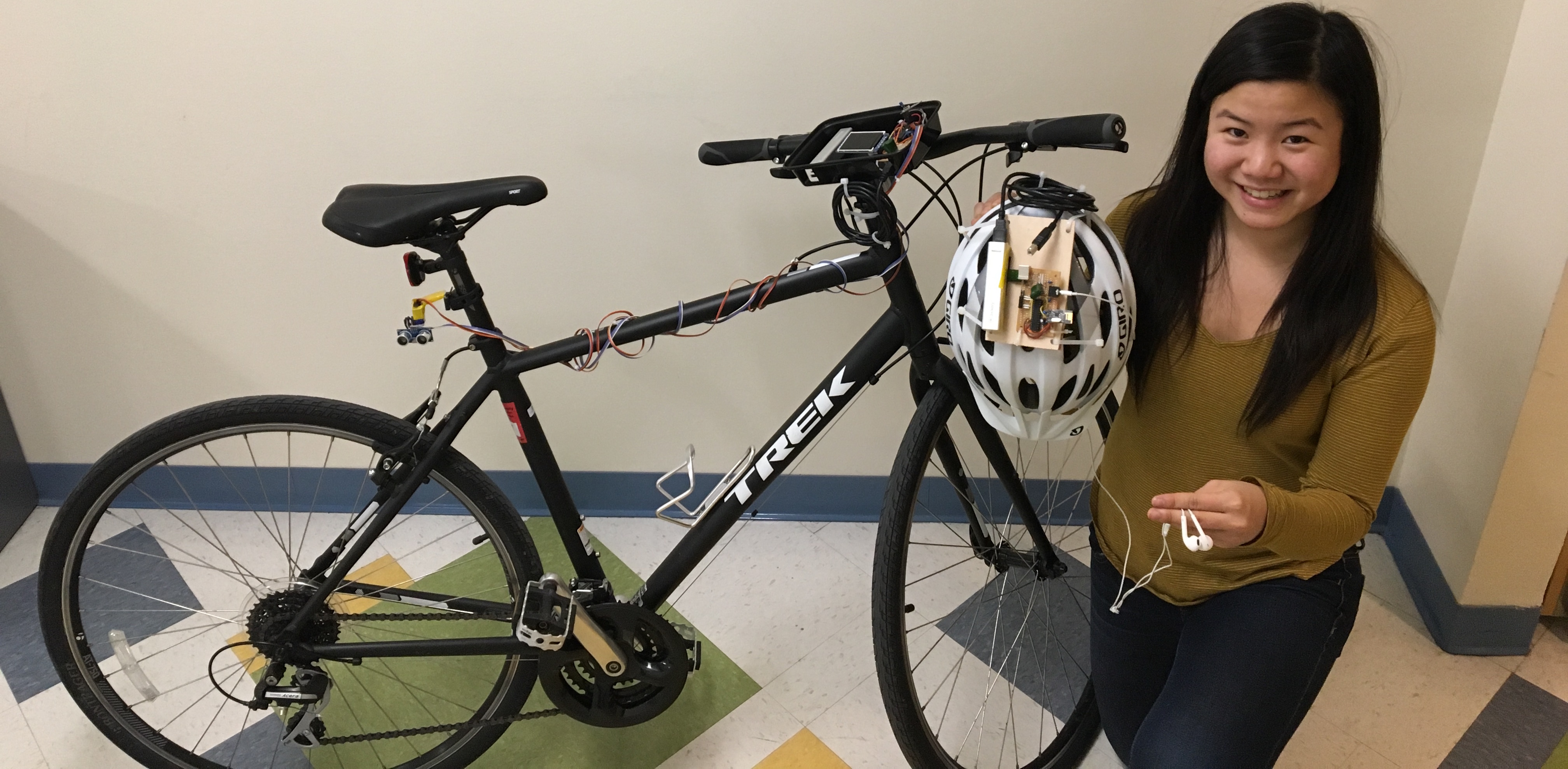
Bike Sonar
Rear-facing sonar with sound localization feedback
Bicycling, either for recreation or for commuting, has exploded in popularity within the past few years. According to a recent survey, over 100 million Americans bike each year. However, only 14 out of the 100 million Americans hop on a bike at least twice a week. The highest cited reason behind Americans' hesitation of everyday cycling is the fear of being struck by a vehicle on the road. The statistics seem to back them up. According to the U.S. Department of Transportation, 45,000 cyclists were injured in traffic in 2015, with 818 being killed on U.S. roads. The issue lies behind drivers’ and cyclists’ inattention to road laws, as well as the lack of effective space between drivers and cyclists. If there was a simple means to incentivize more of the population to commute or exercise via cycling, much of the population could reap enormous health benefits, as well as contribute to decreasing the amount of carbon dioxide spewed out annually by commuters.
We see the inherent risks in cycling, so we wanted to provide a means to address the hazards cyclists see everyday on the road. The U.S. Department of Transportation identified parallel-path events (e.g. cars or cyclists merging lanes) as one of the most common causes of bicycle-motor vehicle accidents. Thus, we decided to create a device that increases cyclists' awareness and enhances their peripheral vision while on the road.
Our project, the Bike Sonar, does just that.
High Level Design
In order to enhance users' awareness around them while minimizing further distractions while on the road, we created a system that would warn users when vehicles were within a certain range (within 4 meters) behind them. Our device consists of two components, both controlled by PIC32 microcontrollers. First, a "bike side" system is mounted on the handlebar frame of the bicycle. This system controls a servo, mounted on the seat post, that sweeps from side-to-side. An ultrasonic rangefinder is mounted to the servo, pointing backwards. The system sends pings from the ultrasonic rangefinder while the servo is sweeping, measuring the distance to the closest object. In this manner, a map of objects behind the cyclist is constructed. On the bike side, a LCD display graphically shows this map, color coded so users can quickly glance down and see if a car is within a close proximity. However, we are aware that even a graphical display may be distracting to users. Thus, our second component uses audio warnings.
Our second system consists of another PIC32 microcontroller mounted to the cyclist's helmet. This PIC32 receives information via a 2.4GHz radio signal from the bike side system containing angle and distance data of potential hazards behind the cyclist. The helmet side system will then generate audio "pings" that actually sound like they are originating from the direction of the potential hazard. The intensity of the pings correspond to the physical distance of the hazard to the cyclist. In this manner, cyclists do not even have to take their eyes off the road in order to know the exact distance and direction of dangers behind them. With this combination of audio and visual cues, cyclists gain confidence and a sense of security while riding and merging on busy roads.
During the development of our project, we had to carefully balance tradeoffs and consider the interface between hardware and software. While we could have utilized the PIC32's processing power to achieve faster computation, draw more detailed images, or obtain a higher throughput of readings, we were constrained by hardware. The HC-SR04 ultrasonic sensors we used could only sample once every 60ms, which provided a strict limit on our throughput. Furthermore, we had to use both hardware and software solutions in order to obtain a robust system. Since our radio communications were very subjective to noise generated by our TFT display, servos, and sensor, we used a combination of threaded code structure, packet acknowledgements, and additional hardware such as decoupling capacitors in order to obtain a stable radio system. Thus, our main takeaway from this project is that we learned how to develop a real embedded system, taking into account tradeoffs and constraints between hardware and software, and using both hardware and software solutions to achieve a final product.
Finally, we verified that our project adhered to legal restrictions, which we discuss further in the Conclusion section. Our main concern was our radio communication system. Our radios operated in the 2.4 GHz Industrial, Scientific, and Medicine (ISM) radio band regulated by the FCC. We verified that our radios operated within the power limitations of the ISM band, which is that the maximum transmitter power fed into the antenna is 30 dBm, and the maximum effective isotropic radiated power is less than 36 dBm. Likewise, while we found commercial products that were meant to warn users of vehicles, our project was the only product we found which focused on sound localization, as well as using an ultrasonic sensor in conjunction with a servo.
Sound Localization
The key technology utilized in our project relies on generating audio signals that sound as if they are originating from a specific lateral angle with respect to the user. Sound localization is a widely studied area. However, the high level explanation behind sound localization lies behind the subtle differences in phase and intensity between our two ears that our brain processes. These two diferences are referred to as the Interaural Time Difference (ITD) and Interaural Intensity Difference (IID). These two near-imperceptible differences both contribute to sound localization. However, for frequencies below ~500 Hz, IID plays a negligible part in sound localization, since these longer wavelengths are diffracted so the intensity differences are minute. On the other hand, ITD, and the resulting phase difference, is the main factor in sound localization.
All the calculations are based of the angle, theta, and maximum sensing range, MAX_DISTANCE, shown in the image below.
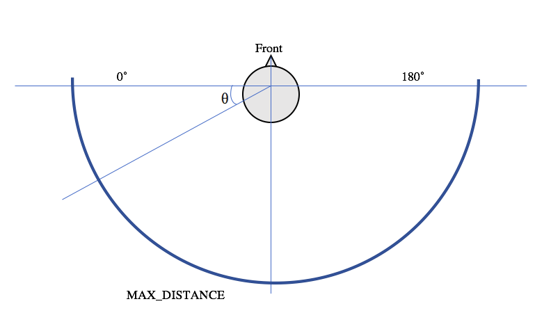
Angle and distance corresponding to head location
The angle of the sensed object is used to determine the time (and phase) difference for the waveforms recieved by the left and right ears. The maximum time delay from one side of the head to the other is the amount of time it takes for sound to travel across the distance between both ears. For the demo, we assumed this maximum delay to be 500us, but this is a parameter that can be easily changed to match a user's head size by changing the definition of MAX_HEAD_DELAY_us in sound.h. For all calculations and sound synthesis, we assume that a positive time difference means the left ear leads. We calculate time difference as a function of the angle and scale this to the maximum head delay. The phase difference used to index into the sine table for DDS is calculated as a function of this time difference. These two calculations are shown below.
// Time difference calculation as a function of theta
time_diff = (int) (MAX_HEAD_DELAY_us * cos(degree*PI/180.0));

// Phase difference as a function of time difference
phase_diff = (int) (((time_diff * sound_freq) / 1000000.0) * two32);
While sound localization at a frequencies below ~500Hz works with just phase difference, to intensify the illusion that sound is coming from a certain location, we scale the amplitude of either the left or right waveforms based on the angle of the object. If the object is anywhere to the left of center, the left waveform is a full amplitude, while the right amplitude increases from half the maximum amplitude to full amplitude as the angle approaches 90˚. The opposite is true if the object is anywhere to the right of center. This calculation is shown in the code snippet below.
// Sound amplitude difference scaler based on theta
amplitude_difference_multiplier = 0.5 * sin(degree*PI/180.0) + 0.5;
Finally, to help the user sense an object's proximity, we scale both the left and right waveform amplitudes linearly to the object's distance. If the object is at MAX_DISTANCE, the amplitude of both waveforms will be 0 and the user will not hear any audio feedback. The calculation is shown below. If the object is out of range, the overall amplitude is also scaled to 0.
// Overall sound amplitude scaler based on distance
amplitude_overall_multiplier = -1.0  * (distance/MAX_DISTANCE) + 1;
The time and phase differences, as well as the sound amplitude multipliers, are used to change the waveform parameters when sound is generated usign direct digital synthesis (DDS) in the ISR. We describe these details the Software Design section.
Hardware Design
As we have described in the High Level Design section, our project is divided up into two systems - each consisting of a standalone PIC32 on a solder board. The circuit schematic for each system is located in Appendix B.
Bike-Side Hardware
The corresponding solder board to the bike-side circuit schematic in Appendix B is shown below. Power is provided via a 5V rechargable 3300 mAh power bank, which is attached via a USB Type B cable to a USB header soldered onto our board. The battery can be easily removed and recharged as it is attached via Velcro. The USB header provides 5V power, which powers both the ultrasonic sensor and the servo. 3.3V is provided to the rest of the system via a MCP1702 3.3V LDO. The PIC32 is set up in its standalone configuration according to the circuit provided by this blog post cited in the appendix. The radios that we are using in this lab are nRF24L01 radios, which is connected to the PIC32 as shown in the schematic in the appendix. The TFT display is a 2.2" TFT LCD from Adafruit. Likewise, the connections are shown in the schematic, and is referenced from the ECE 4760 website.
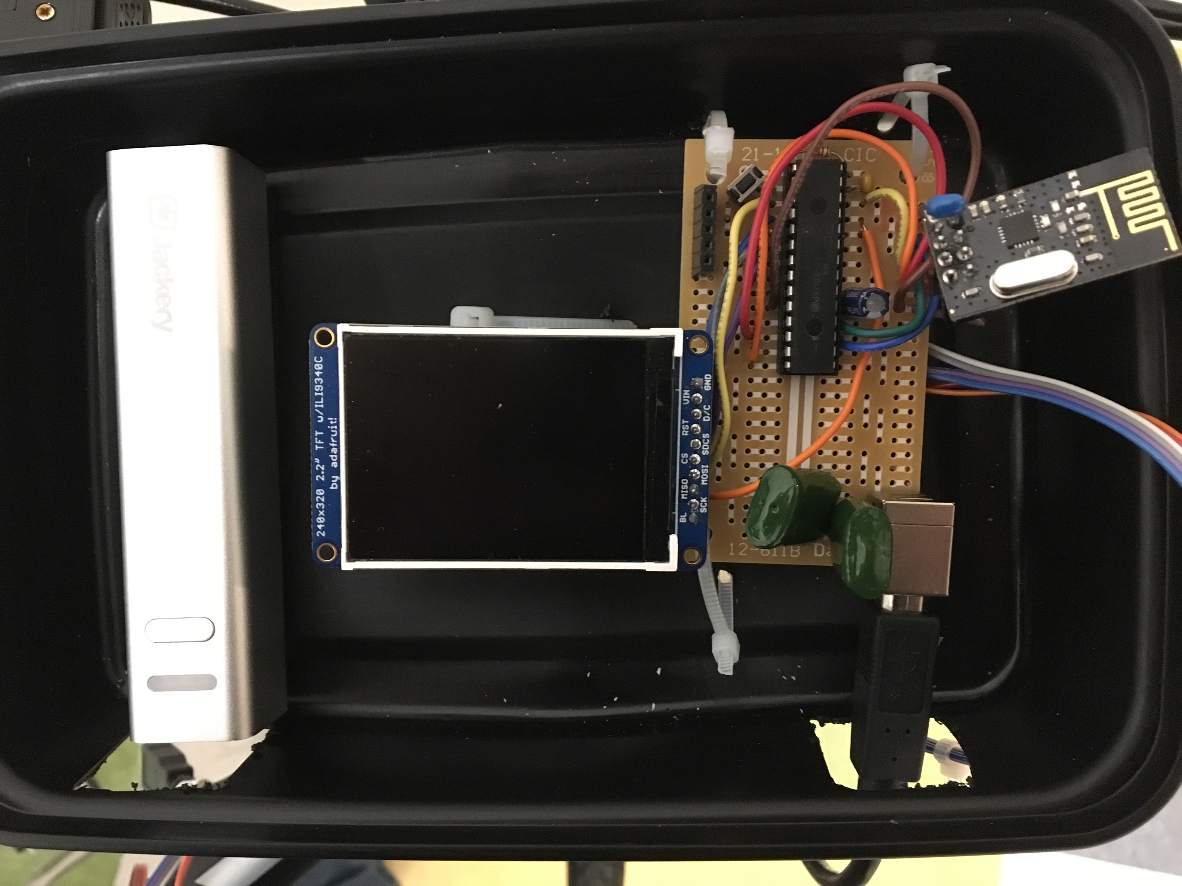
Bike-Side Solder Board
The connections off the board to the ultrasonic sensor and servo are made via physical connections. However, in the future, another standalone PIC system with a radio could be used instead. The attachments for the ultrasonic sensor and servo are shown in the figure below.

Side view of Bike System
Helmet Side Hardware
The circuit schematic for the helmet side board is shown in Appendix B. Furthermore, a image of our solder board is shown in the figure below. As with the bike side system, the board contains a PIC32 standalone system. Furthermore, the power source, as well as the 3.3V MCP1702 LDO and the Nordic nRF24L01 radio is the same. The difference, in terms of hardware, is that we are using a 12-bit DAC (MCP4822) in order to generate our sound. The DAC is connected to the PIC32 via SPI. There are two output channels on the DAC, each connected to the right or left channel on a 3.5mm audio jack. To reduce clipping on the headphones, a 1 kOhm resistor is placed in series with a 10uF capacitor on each of the connections to the audio jack, as done in a previous ECE4760 project that involved playing audio through headphones.
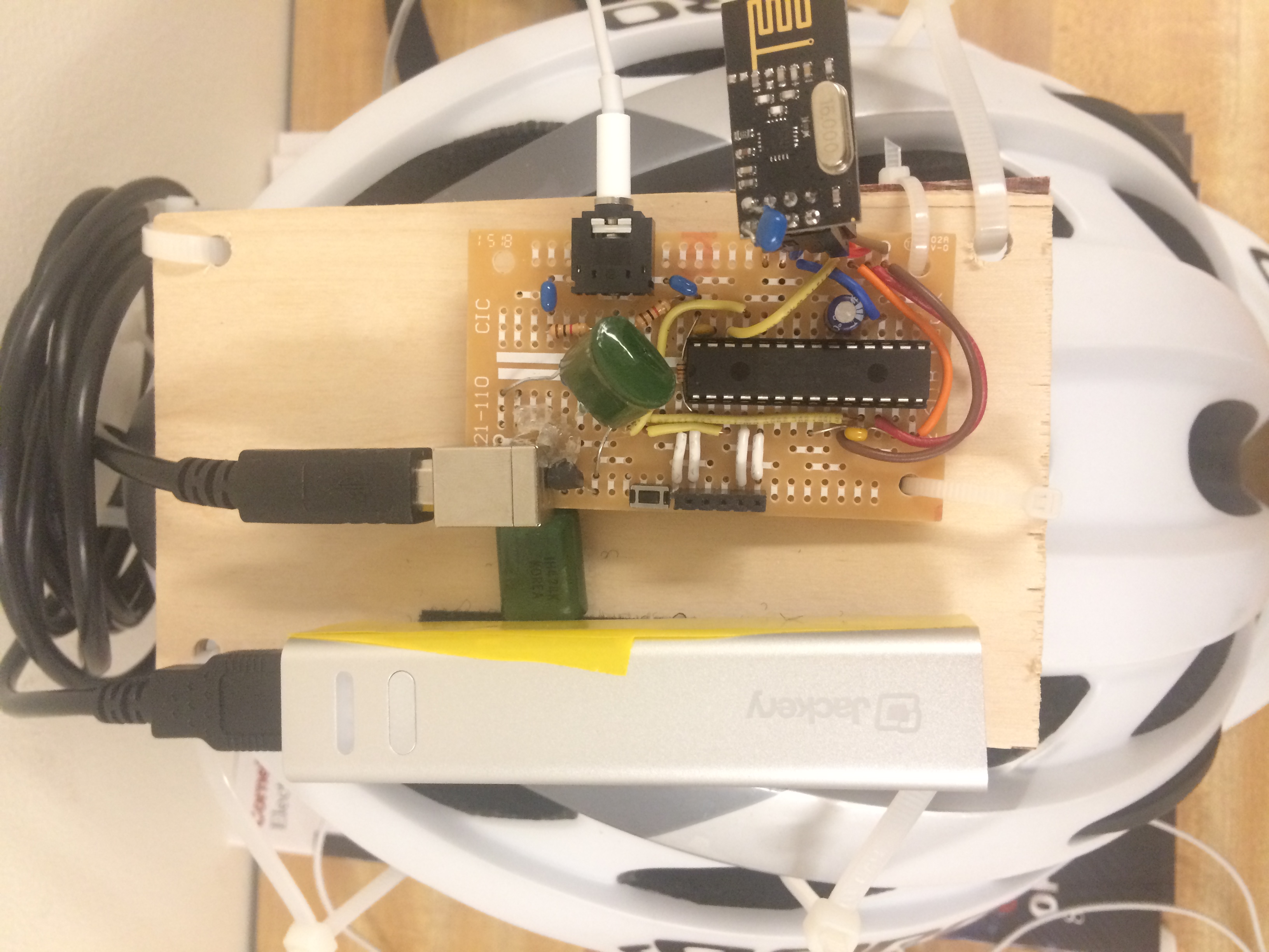
Helmet-Side Solder Board
Software Design
We created separate projects to be loaded on to the PIC on the bike side and the PIC on the helmet side. These two standalone systems communicate via radio. Functions for the various subsystems are separated libraries to make our code modular and easier to understand. The bike side includes a servo library, graphics library, and ultrasonic sensor library. The helmet side includes a sound library. These libraries contain functions to initialize the correct peripherals and timers for each component. Both the helmet and bike side contain the radio library, written by Douglas Katz and Fred Kummer. The organization of both the helmet and bike software showing all the relevant source code and libraries is listed below. The program listings are linked to in Appendix C. Implementation details for each subsytem are also described below.
- Bike.X
- main.c (main)
- config.h; Syed Tahmid Mahbub and Bruce Land
- servo.h/.c
- ultrasonic.h/.c
- graphics.h/.c
- nrf24l01.h/.c ; by Dave Katz and Fred Kummer
- radio.h/.c
- tft_master.h/.c; by Syed Tahmid Mahbub
- tft_gfx.h/.c
- pt_cornell_1_2.h; by Bruce Land
- glcdfont.c
- Helmet.X
- main.c
- config.h; Syed Tahmid Mahbub and Bruce Land
- sound.h/.c
- nrf24l01.h/.c ; by Dave Katz and Fred Kummer
- radio.h/.c
- tft_master.h/.c; by Syed Tahmid Mahbub
- tft_gfx.h/.c
- pt_cornell_1_2.h; by Bruce Land
- glcdfont.c
Servo motion with Output Compare
Servos are controlled with pulses of varying widths, as shown in the image below. .
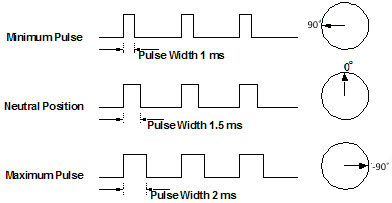
Servo pulses corresponding to angles. Image from ServoCity.com
We control the servo with an output compare module that generates a pulse with a 20ms period using timer 2. The output compare is set to pulse width modulation (PWM) mode. To change the angle of the servo, we change the duration of the high pulse. The image above shows the theoretical pulse widths typically used to control servos, but through testing, we found that sending pulses of those widths to our servo did not produce the desired angles. To account for this, we callibrated the by varying the pulse width until it turned to the correct angles. The following excerpt of code maps an angle from 90˚ to -90˚ to a high pulse duration of 680us and 2400us, respectively. At a pre-scaler of 1:64, these values correspond to 420 and 1500 timer ticks, respectively.
// Maps angle of servo to value to be loaded into timer
timer_val = (int) (-(1080/180.0)*deg + 960);
Measuring Distance with Output Compare and Input Capture
As shown in the timing diagram below, ultrasonic sensor must recieve a 10us pulse on the trigger pin to send an eight-cycle sonic burst at 40kHz, which it uses to measure distance. The echo pin will recieve a pulse of some duration, which proportional to the distance of the object.

Ultrasonic sensor timing diagram from datasheet
The 10us is output with another output compare module and the echo pulse is measured with an input compare module for accurate timing. Both modules use the same timer. An input capture module is configured to capture on every edge. For every distance measurement, a 10us pulse must be sent out. This is done by opening an output compare module to send a one-time pulse of 10us. Immediately after the pulse is sent out and prior to recieving the echo pulse, the timer is reset to 0x0000. About 500us after recieving the trigger pulse, the sensor will recieve an echo. The input capture will trigger an ISR on both edges, which determines the length of this echo pulse. Within the ISR, we read the level of the input capture pin to determine if the ISR was triggered by a falling or rising edge. The value of the capture register is recorded for both edges, but the length of the pulse is calculated by finding the difference between these two values only when the ISR is triggered on a falling edge to ensure that we only measure the length of the high pulse. This value is recorded in timer ticks, which, at a pre-scaler value of 1:64, are 1.6us each. The length of the pulse is converted into a distance with the following formula:
// distance = (high level time) * (speed of sound)/2
distance_cm = (capture1_delta * 1.6) / 58;
Generating Localized Sound Bursts with Direct Digital Synthesis
DDS is a method of generating analog waves, in this case, sine waves, by taking digital values and converting them to analog signals. To produce sine waves of different frequencies, our implementation of DDS reads out digital values from a 256-element sine table at various frequencies by indexing into the table with a phase accumulator at varying increments within an ISR. Though DDS is capable of generating a wide range of frequencies, we only need to produce one frequency for sound localization. Each phase accumulator is a 32-bit int. The accumlator is shifted right by 24 bits because only the top 8 bits are used to index into the sine table. The incrementing accumulators simulate a rotating phasor scanning one period of a sine wave. The frequency of the DDS-generated wave is determined by the rate at which we step through the sine table. This is varied by setting the phase accumulator increment to a value corresponding to the desired frequency. Since the accumulators are ints, they will overflow when they reach a value of 232. The frequency of the generated sine wave, Fout , depends on how many times the sine table is traversed completely every second, which can be varied by making the phase increment value bigger or smaller. For a given sample frequency Fs, determiend by the rate at which the ISR is triggered, Fout = (Fs * increment) / 232. We generate the sine table array once in main() using floating point arithmetic to make recalling sine values easy in the ISR. Similarly, we determine the increment necessary for the desired frequency in main() and store these in a table for quick look-up in the ISR. The ISR is triggered by an overflowing timer. Since the ISR is continuously entered, a flag is necessary to control when sound is played and when it is not.
To create the illusion that a sound is coming from certain angles around a user's head, we generate two sine waves of the same frequency but slighlty out of phase. As such, we must index into the same table twice, but with two 'phase accumulators' that are incremented with the same amount but are slightly offset from each other. This offset, or phase difference, is calculated based on the angle of the detected object. This calculation is explained in the High Level Design section. The values read from the sine table range from -2047 to 2047, so they must be shifted up by 2048 to match the values the 12-bit DAC can take. Prior to sending these values to the DAC via SPI, we manipulate them a bit more to create more convincing sound localization illusion and give the tone bursts a nicer sound. To enhance the sound localization effect and scale sound amplitude to object proximity, we multiply the sine table values by both amplitude multipliers shown in the High Level Design section.
In order to create more pleasant sounding tones, we chose to use a linear ramp to gradually transition the amplitude of the sound bursts from maximum to minimum and vice versa. Each tone burst ramps up to full amplitude in 8ms and back down zero in another 8ms. We determine how to scale the amplitude by keeping track of each tone's duration in global variable at the time of every DDS sample. The variable is incremented by the period of the ISR in microseconds (us). For our chosen sample frequency and implementation, the ISR period is 2500 cycles, or 62.5us with a 40MHz clock. To minimize floating point arithmetic in the ISR, we increment the tone duration variable by 62. The amplitude of the sine wave data is scaled linearly or not scaled according how long the tone has been playing. For sound localization, these sound enevelopes also needed to be time delayed in accordance with the phase delay. To do this, we separately keep track of both the left and right tone durations and perform the same ramping scheme on both.
Radio Communication
Communication between the two PIC32s was facilitated using two Nordic nRF24L01 radios operating in the 2.4GHz ISM band as described in the Hardware Section . We used the nrf24l01 Library in order to actually control the radios. In more specific detail, the library allowed us to fine-tune how our radios functioned. Importantly, we set up the radios to auto acknowledge each packet sent, with 10 attempts of retransmissions. Furthermore, each packet had a fixed length of 4 bytes. In our project, we only sent packets from the bike side to the helmet side system. However, the hardware allows for full duplex transmission in the event of future additons to our project. The first byte in each packet is the transport layer header, informing the helmet system about the information included in the remainder of the packet. Currently, we simply use the ASCII value of 'd' as the header for distance and direction packets, and we use the ASCII value of 'n' as the header for a out-of-range packet. For our distance/direction packets, the second byte contained the direction of the measurement, ranging from 0 (full left) to 180 (full right). Finally, the third and fourth byte contained the distance measurement as a 16-bit value.

Distance/Angle Packet Format
On each PIC32, we used a protothreads thread to run the radio communications. Each thread effectively acted as a FSM. The FSM diagrams for both the bike and helmet side radio code is shown below. At a high level, the bike radio thread first began by establishing a connection, by sending a packet, to the helmet thread. When this was successful, the bike thread then fell into a loop. Each loop began with a distance measurement at a pre-determined angle. Given these measurements, a new packet is created with contents being formatted depending on the if the reading is greater than or less than the maximum measurement range. Next, the FSM checks to see if there is an echo of the previously-sent packet from the helmet side. If there is no echo, the packet is transmitted and the angle is not incremented. If there is an echo, the packet is transmitted and the angle is incremented. This ensures that in the event of a lost packet, we do not miss a reading at a given angle. We then return to the top of the loop and repeat this sequence.

Bike Side Radio FSM
The helmet side FSM is much simpler than the bike side. Effectively, the helmet side simply waits for packets to arrive. When a packet does arrive, it checks the header to see if the packet contains valid information. If there is valid information, the sound corresponding to the packet's angle and distance measurements is played. Finally, the packet is echoed back to the bike side, and the process repeats.

Helmet Side Radio FSM
Graphics
A graphical display was mounted on the handlebars in order to visually display the map of the user's surroundings. A sample image of the display is shown in the figure below. The tft_graphics library was used in order to create the graphics shown below. The graphics code runs in a thread that is called every ~100 milliseconds. Every time the thread is called, the current angle and distance measurement is displayed on the TFT screen. A 15 degree cone is drawn out, with our current angle centered on the cone, that emanates from the top center of the screen. The corresponding distance is shown in two ways. First, the size of the cone linearly corresponds to the distance from the ultrasonic rangefinder. As shown below, the range is from 0cm to 360cm, corresponding to the outer green semicircle. Secondly, the color of the cone varies based on distance. In order to encode our color, a scale, we varied the red component of our color from 0 to 255 corresponding to the distance from 0 to MAX_DIST/2. We varied the green component of our color from 0 to 255 corresponding to the distance from MAX_DIST to MAX_DIST/2. In this manner, we were able to visually display our sensor readings with red corresponding to a close-proximity hazard and green corresponding to farther away objects. Thus, users are able to quickly glance at the screen in order to see any objects that are within a close proximity.
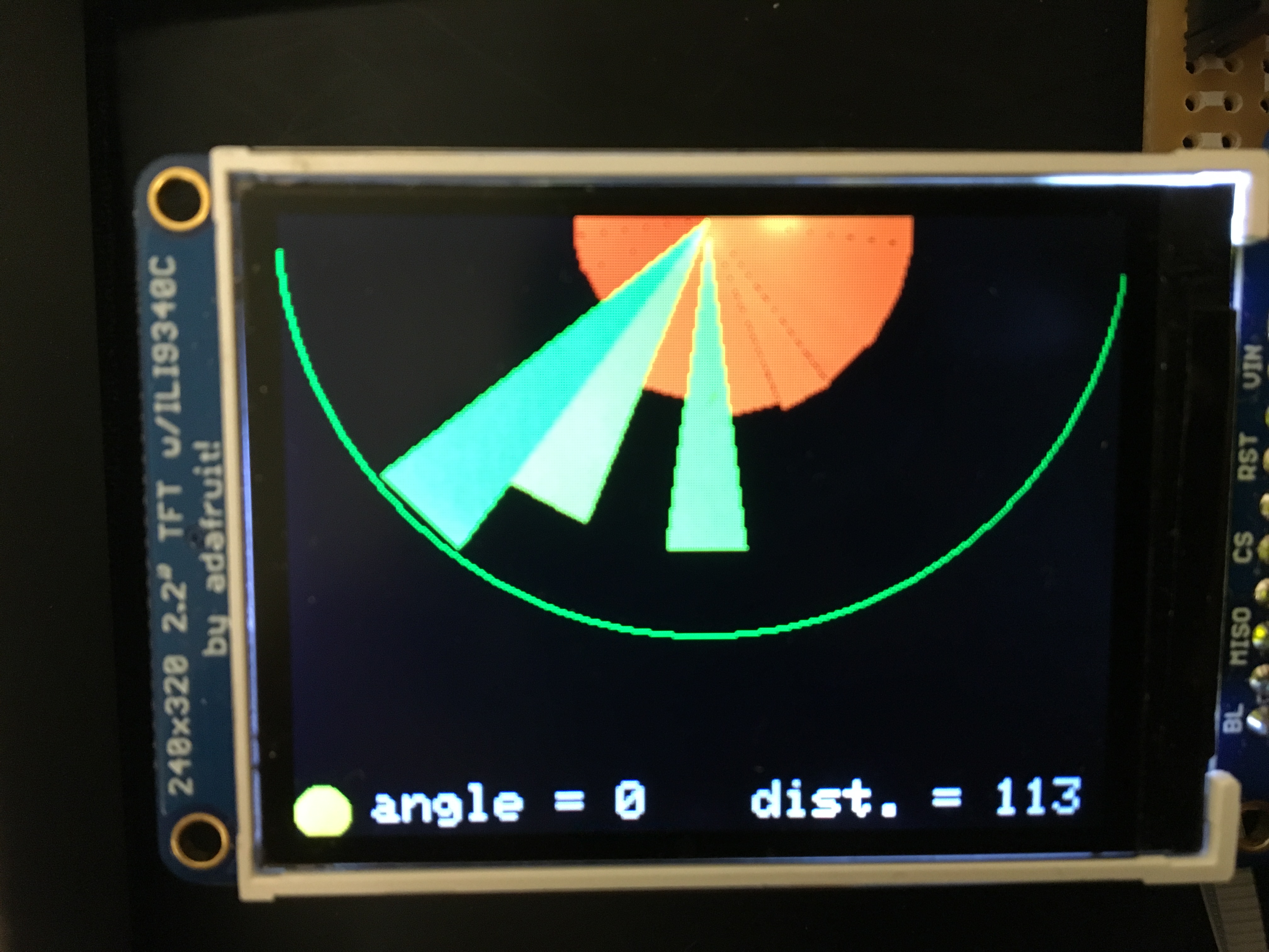
Graphical TFT Display
Results
Measuring Distance
When testing the ultrasonic sensor, we found that it produced the best results when pointed at hard, reflective, flat surfaces. The image below shows the 10us trigger pulse on channel 1 and the echo pulse for an object about two meters from the sensor on channel 2. As we moved the object towards and away from the sensor, the echo pulse would shrink and grow. We found that 360cm seemed to be the maximum range of the sensor.
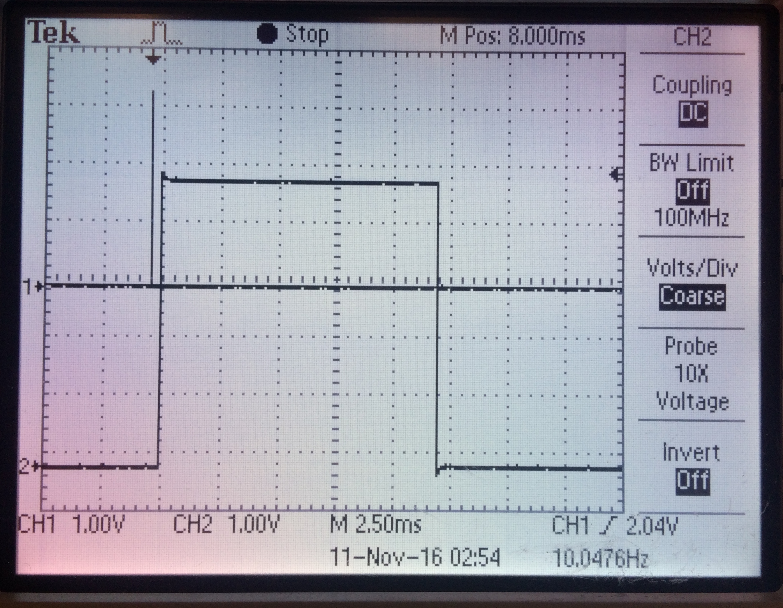
Ultrasonic trigger and echo pulse for object at ~2m
Sound Localization
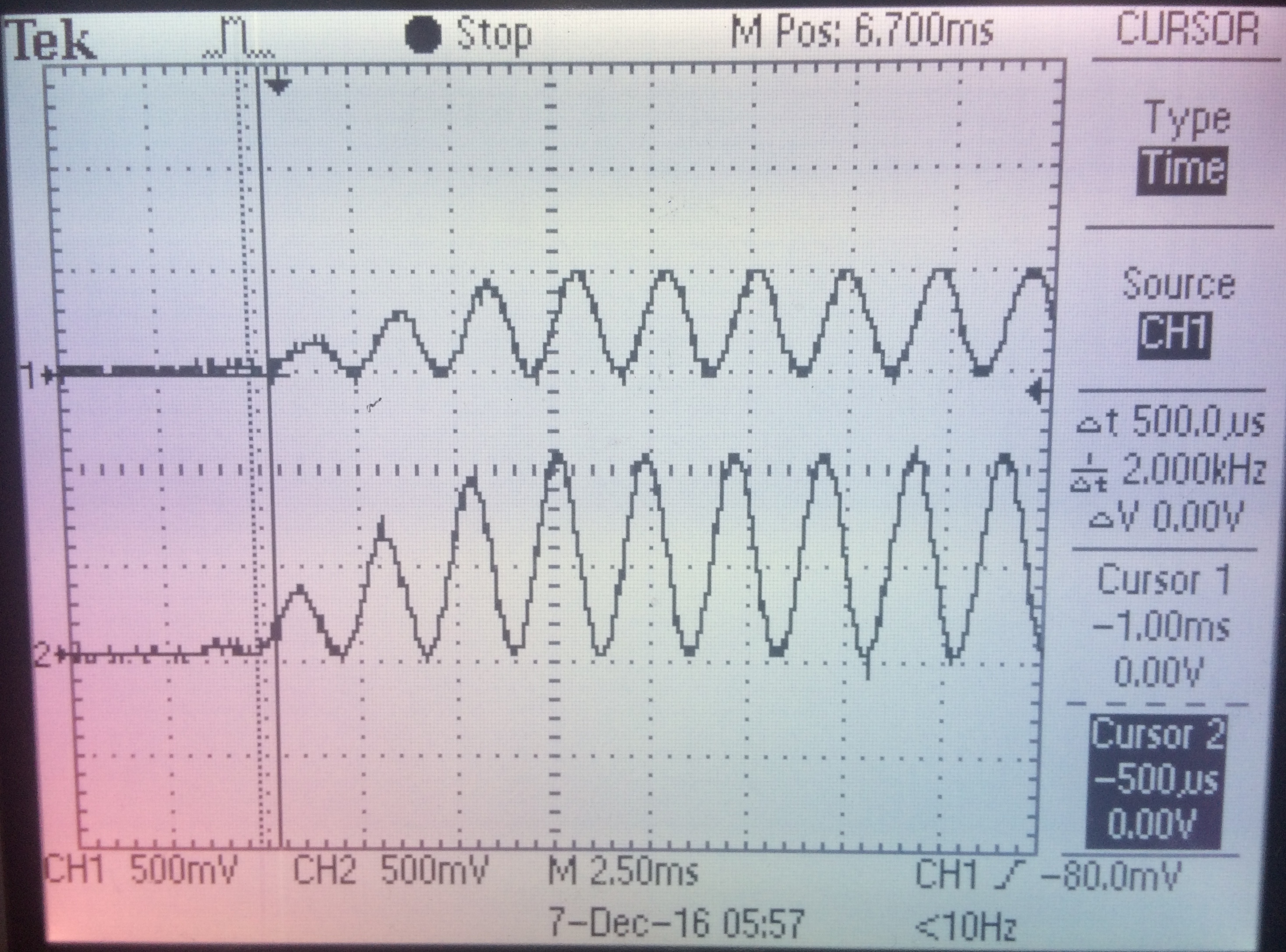
We first tried sound localization using a 300Hz, 250ms sound bursts played from the leftmost and rightmost angle. While these burts were slightly differentiable from each other, we wanted a more convincing illusion. To achieve this, we introduced a small intensity difference based on the angle of the object. The images below show sound localization waveforms at varying angles and distances with both phase and intensity difference. The images also illustrate the time delay in the sound envelopes. In all three images, channel 1 scopes the right ear and and channel 2 scopes the left ear.
Upward ramp of sound waveform - object is 200cm away from biker, directly left of biker. Channel 2 is waveform heard in left ear. The left waveform leads the right waveform by 500us. The intensity of the left waveform is twice that of the right waveform.
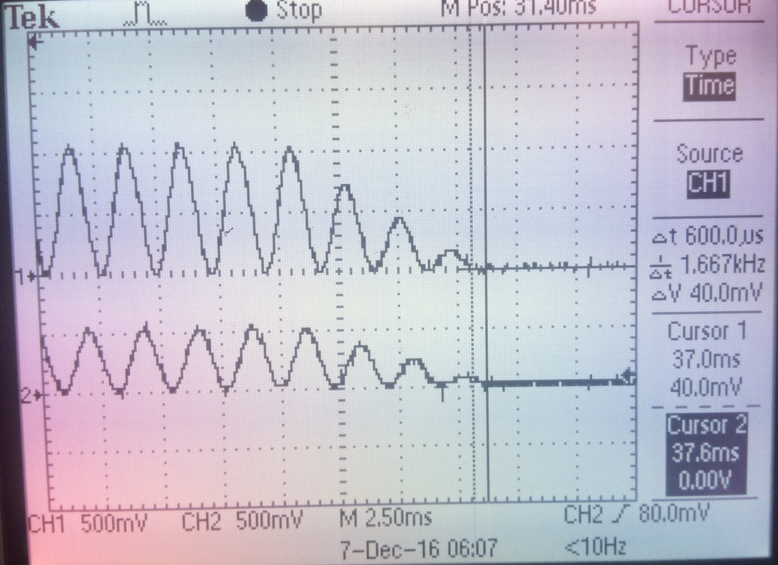
Downward ramp of sound waveform: object is 200cm from biker, directly right of biker. Channel 2 is waveform heard in left ear. The right waveform leads the right waveform by 500us. The intensity of the right waveform is twice that of the left waveform.
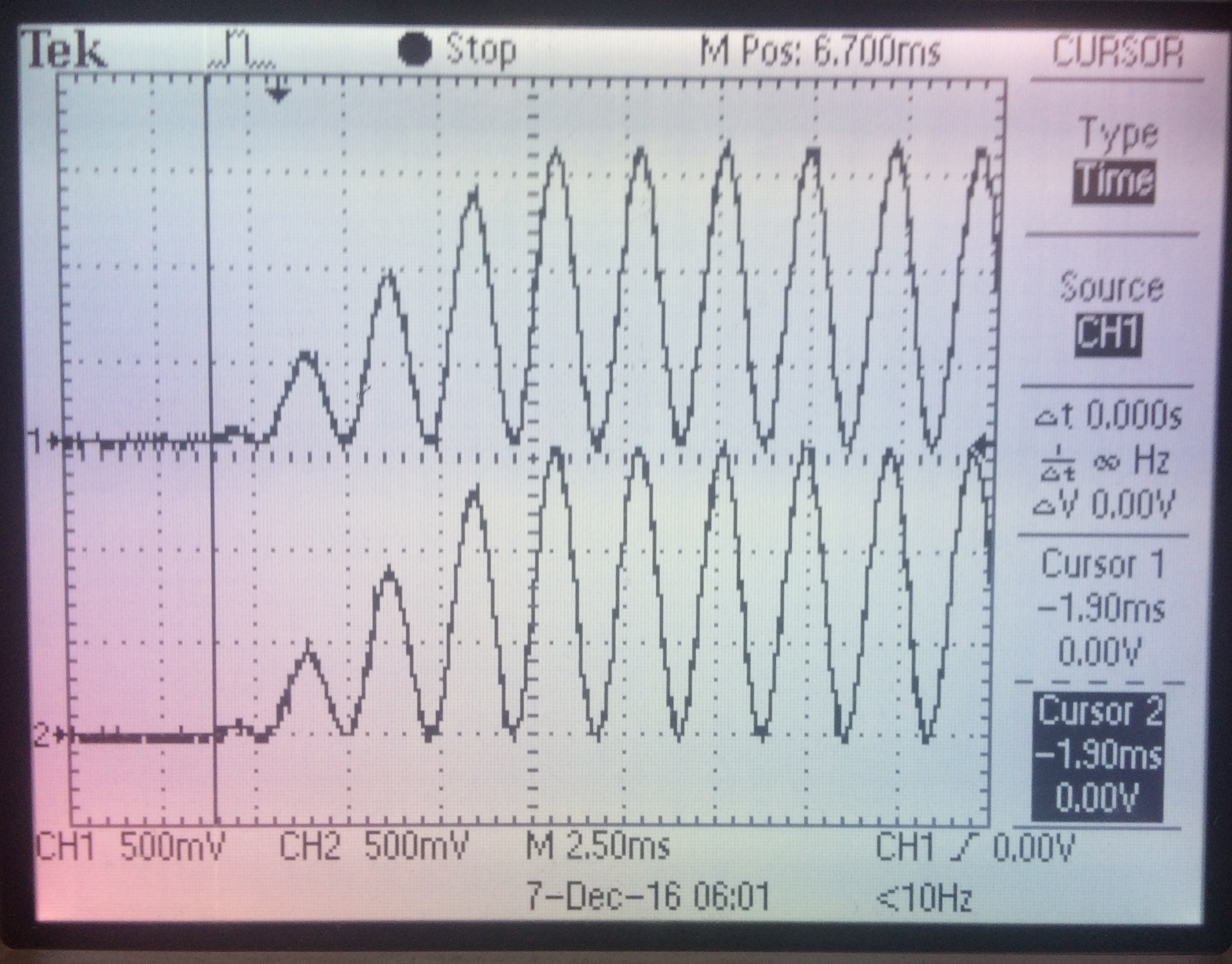
Downward rampound sound waveform: sound source is 100cm from biker, directly right of biker. Channel 2 is waveform heard in left ear. The two waveforms are in phase with each other and have the same intensity. Since the object closer than in the previous two images, these waveforms have a larger maximum amplitude of about 1.5V.
Through headphones, the overall sound localization with amplitude adjustments is convincing. The user is able to discern the general direction from which a sound appears to originate from.
Radio
The radio system gave us the most trouble out of all of the components in our project. While the radios worked fine solely by themselves, after integrating it into our overall design, we experienced many problems with packets being dropped and the radio communication freezing entirely. After many hours of debugging, it seemed as if there was not only one cause behind the unreliability. Instead, it seemed that noise from all of our other components (e.g. the TFT screen and the ultrasonic sensor) caused us to drop packets. To alleviate this problem, we incrementally developed both improvements in hardware and software. In hardware, we placed multiple decoupling capacitors throughout our circuit in order to provide a steady voltage to the radio. Furthermore, we attempted to isolate the SPI clock lines across our circuit by routing wires away from the two SPI clocks. Finally, we added a small capacitor on the trigger line of the ultrasonic sensor to remove the sharp peak that occurs when we want to obtain a reading. While these solutions seemed to alleviate the problem, it did not fix it. Thus, we also added changes in software in order to make our code more robust. For example, we set the radios to send auto acknowledgements to each other. We also created the FSM as described in the Software Design section that provides further reliability to our system. With both software and hardware solutions, we were able to obtain a consistent connection between the two sides, albeit at a slower transmission rate. There is a possibility of interference at 2.4GHz, so to avoid this, we made sure to use a different channel than other lab groups who also used radio communication.
Overall System
The overall system includes both an audio feedback and visual display suitable for demonstration purposes as well as practical use. The visual sonar feedback clearly displays the readings. In order to mitigate distractions due to cyclists constantly looking at the display, we used both a size and color encoding for distance, so cyclists can quickly see and hazards around them. Furthermore, in order to allow the cyclist to devote his or her full attention to the road, our audio feedback system successfully provides localized sound pings warning of any potential hazards. When used with non-noise blocking headphones, the user is still able to hear external noise. With this project, we were able to provide a proof-of-concept for a potential product. We created a system that translates ultrasonic distance readings into both visual and audio warnings. Furthermore, we were able to create localized sound on a PIC32 using DDS. While the system works well in lab settings, it is likely still unsuitable for use in a realistic road biking scenario. With further improvements in radio reliability (via more robust circuitry and software), faster sweep speeds (via additional sensors or faster servos), and improved water-resistant packaging, we hope to obtain a road-ready product. Our project is demonstrates that such a final product is indeed possible.
Conclusions
We are happy with the performance of the overall system for prototype demonstration purposes, but acknowledge that many improvements must be made to bring this project into practical situations. At the start of the project, we envisioned a smoother-functioning system, but we ran into obstacles along the way that prevented us from fully achieving this. The largest issue we had to overcome was maintaining consistent radio communication. We found the way to do so was to slow down transmission rate of packets by slowing the rate of the servo and ultrasonic readings. However, we believe that this problem could be mitigated via more robust circuitry or by using additional sensors. We spent a lot of time debugging the radio but are ultimately proud of our solution to prevent the radio from timing out. For intellectual property considerations, please refer to our discussion in High Level Design.
If we were to continue working on this project, we would take steps to make it more suitable for use by improving distance sensor accuracy and servo sweep speed. The motivation behind our project was to detect moving cars, so we would like to have our system accurately detect quickly-moving objects. We also would like to further enchance the auditory feedback by pitch shifting a sound as a detected object moves towards the user to mimic the Doppler effect.
We confirm that our project adhered to legal restrictions. Our main concern was our radio communication system. Our radios operated in the 2.4 GHz Industrial, Scientific, and Medicine (ISM) radio band regulated by the FCC. We verify that our radios operate within the power limitations of the ISM band, which is that the maximum transmitter power fed into the antenna is 30 dBm, and the maximum effective isotropic radiated power is less than 36 dBm.
As electrical engineers, we have a responsiblity to adhere to the IEEE code of ethics. Our Bike Sonar aims to improve the safety of bike users. The system would ideally be used in real road-biking scenarios, but the project is currently only a prototype. As statement 1 in the code of ethics says, we must "disclose...factors that might endanger the public or the environment," so we advise against using the current Bike Sonar system in a situtation involving cars. We are very proud of our project, but we do not believe we have, in any way, made false claims about the results. We hope that our documentation can help others better understand the technology behind microcontroller design, and we welcome any honest criticism and feedback readers may have for us. Finally, we would like to thank all who contributed to our project, either with pre-existing code or verbal help. All contributors and references have been cited in Appendix F.
Appendices
Appendix A: Website and Video Approval
The group approves this report for inclusion on the course website. The group approves the video for inclusion on the course YouTube channel.
Appendix B: Schematics
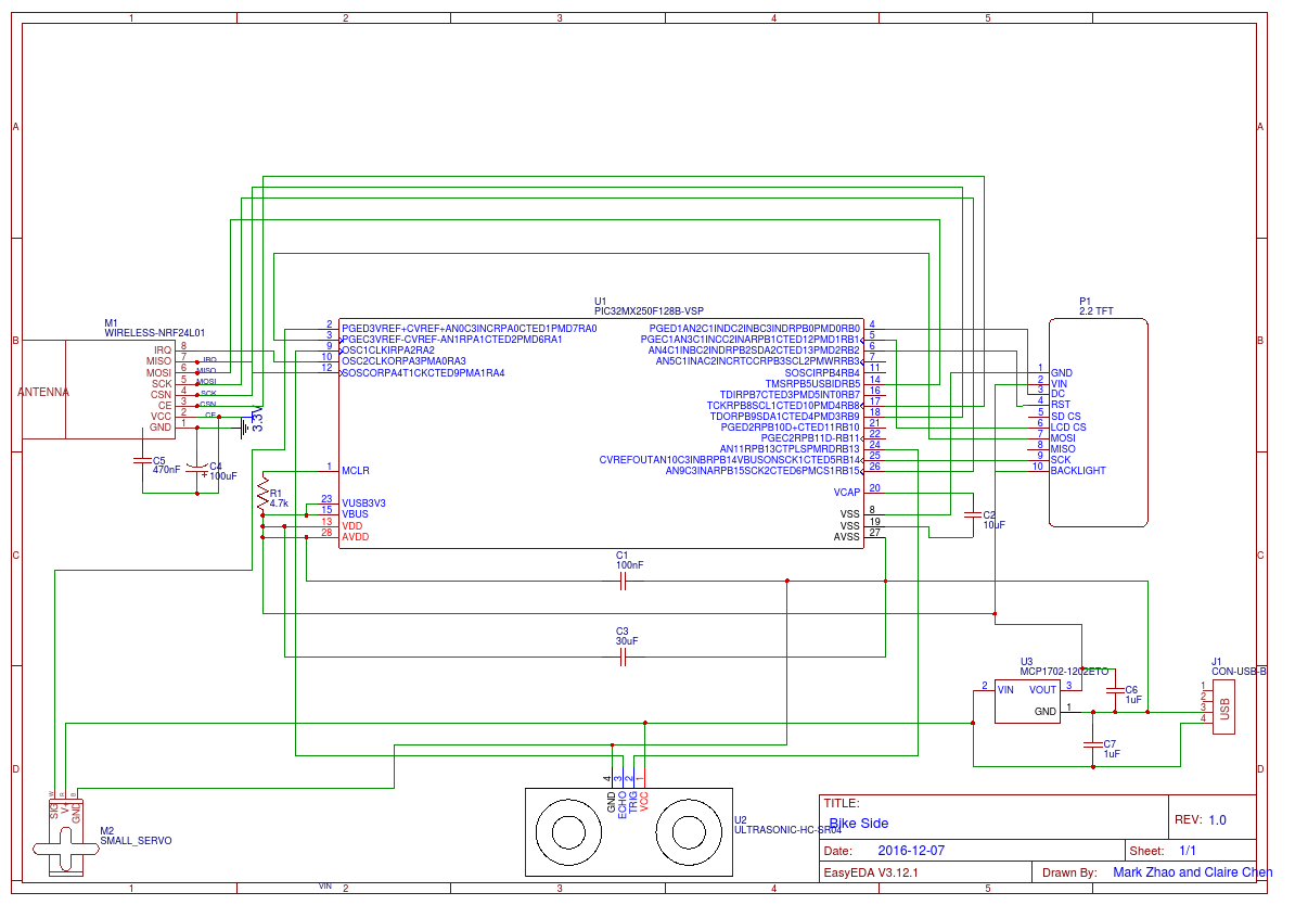
Bike-Side Circuit Schematic
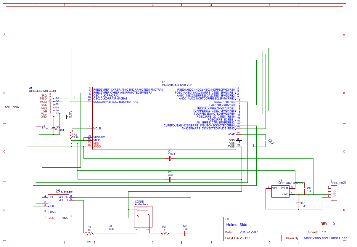
Helmet-Side Circuit Schematic
Appendix C: Code
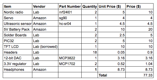
Appendix D: Cost Details
Appendix E: Work Distribution
Claire:
For the project, I worked on servo control (with Mark), distance measurements using the ultrasonic sensor, and sound localization. I soldered one of the standalone systems. Mark and I worked on software integration together. For the lab report, I worked mostly on writing software design, results, and conclusions.
Mark:
For this project, I workd mostly on the bike side of the system. With Claire, we built a servo library that allows us to produce accurate servo commands. I then worked on creating the graphical display. I spent a considerable time setting up, coding, and debugging the radio communication link between our two systems. Finally, Claire and I worked on software integration together. For the lab report, I worked mostly on writing the introduction, high level design and, hardware design (including schematics).
Appendix F: References
We would like to thank Prof. Bruce Land and TA Matthew Filipek for their help throughout the semester. All the datasheets and references we used throughout this project are listed and linked below.
Resources
Sound localization background:
acousticslab.org
nRF24L01 documentation:
PIC32 student project
Biking Trends:
article
Bicycle crash types:
paper
PICkit 3 tutorial:
website
Datasheets
12-bit DAC: MCP4822
Servo: Tower Pro SG90
Ultrasonic sensor: HC-SR04
Radio: nRF24L01
3.3V Regulator: MCP1702