Hardware

Our hardware consisted mainly of the Seiko G321D LCD panel, ADXL 210 accelerometer, KL100 linear potentiometer, rotary potentiometer, custom PCB board, buttons and our packaging of all the items in a box.  The schematic of the hardware design is shown in the diagram below.

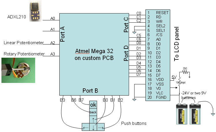
Fig 1.  Overall Hardware design

The ADXL210 is a two-axis accelerometer that goes up to ±10g.  We originally wanted to use a differential method of getting the acceleration from two accelerometers (MMA 3201 from Freescale) but finally decided against it when they gave very low resolution and did not seem to work well with the differential ADC option in the Mega32.  Then we used decided to use the 2g accelerometer ADXL 202.  However, after many testing attempts, we found that if we were to hit the ball really hard, the accelerations would go beyond 2g.  Hence, we wired up the three accelerometers and finally decided to use only the 10g accelerometer, as we were not strong enough to hit above 10g.

Software

Coded Ball Physics

Since there are a total of 16 balls in the Full Game mode and up to 6 balls in the Training mode, we realize it is efficient to code each ball as an object with different variables, such as velocity v, vx, vy, theta, x and y positions etc.  The cueball takes on ball[0], ball number 1 ball[1] and so on, so that a for loop can be implemented easily when required.

For the purpose of simple ball playing alone (without having a full game implemented), all we need are 3 states within the task playgame, which is executed once every 100 ms.  These 3 states are cuestick, whiteball and ballhit.

Cuestick is the state that, as the name suggests, involves only the cuestick.  This state primarily interacts with the player, to obtain 3 main parameters through A-D conversion.  A-D conversion takes place in the task readADCs, which is executed once every 33 ms.  In this task, ADMUX is varied such that readings are taken from the accelerometer, the rotary potentiometer, and the linear potentiometer in sequential fashion.  It is assumed in this game that the position of the cuestick takes reference from the cueball. Through some simple calculations, these ADC readings are converted into the parameters cuetip, cue_theta and a, where cuetip represents the distance of the cuetip from the cueball, cue_theta represents the direction of thrust of the cuestick, and a represents the acceleration of the cuestick. 

cueTip=(linear_adc/10) ;             //position the tip of the cue

cue_theta= PI-(( (float)rotaryADC )*2*PI / (float)rotaryMax);

 a=(abs(maxaccel - (total_samples/samNo) )*200 )<<8; //to get from actual data
 

Using the values cuetip and cue_theta, the cuestick is drawn in real time on the LCD screen.  When the value of cuetip gets below a certain threshold value, which we set as 10, it means that the cuestick has hit the cueball and it is time for the cueball to move.  At this point, the state machine enters the state whiteball.

The whiteball state is concerned with the motion of the cueball alone.  For the very first time that the whiteball state is entered, an impactflag is set, so that we can determine the initial velocity of the cueball.  When the impactflag is reset to 0, the velocity is reduced by incorporating a drag force.  Each time velocity is determined, it is essential too to calculate its components vx and vy, through cosines and sines of the theta value.  From these velocity components, we can calculate the new value of x and y, defined as newx and newy.

ball[0].vx = mfix(ball[0].v, cosT(ball[0].theta) );

ball[0].vy = mfix(-ball[0].v, float2long(sin(ball[0].theta)) );

ball[0].newx = (ball[0].x + mfix(ball[0].vx,dt));       //new temporary x position

ball[0].newy = (ball[0].y + mfix(ball[0].vy,dt));       //new temporary y position

To detect collision with the sides of the table, a function called hitTable is called.  If newx or newy is beyond the table boundary, we reset newx or newy at the boundary and reverse the velocity component.  Code for collision with one of the table side is shown below.

//detects collision with right side of the table

if ( (ball[cnt].newx >= xtablemaxLong ) && (ball[cnt].newy > pocket) && (ball[cnt].newy < (ytablemaxLong-pocket))  )

begin

ball[cnt].vx = ball[cnt].vx*-1;

ball[cnt].newx = (xtablemaxLong)-(1<<8);

ball[cnt].theta=PI-ball[cnt].theta;

end

To detect collision with the object balls, a for loop is performed on the 15 object balls.  Using Pythagoras’s theorem, if the distance between the centre of the cueball and any object ball is less than or equal to the ball diameter, it means that the balls have collided.  In that case, we jump from the whiteball state into the ballhit state.

for (n=1;n<=ballsPlayed;n++)  //collision detection with the other balls

         begin

               diffX=(ball[0].newx - ball[n].x);    

               diffX=(mfix(diffX,diffX))>>8;       //make them into actual numbers

               diffY=(ball[0].newy - ball[n].y);

               diffY=(mfix(diffY,diffY))>>8;       //make them into actual numbers

               if( ( diffX + diffY ) <= diameter3 )

              begin       // to prevent 2 balls from overlapping

                   firstHit=0;          //reset firstHit flag

                   state=ballbreak;

              end                       

      end

Ballhit state essentially cycles through all 16 balls through a for loop, and takes turn to determine the new x and y positions of each ball in each step of the loop.  Like the whiteball state, the ballhit state incorporates the same collision detection, hitTable and velocity reduction algorithm.  In addition, the ballhit state on collision determines the velocity and direction the 2 balls will move in after impact.  This is done assuming conservation of linear momentum, as well as a few trigonometric equations, as explained under High Level Design --> Background Math and Physics.

Each time a newx and a newy position is calculated, we undraw the ball’s old position on the screen through the drawball7x7 function.  Similarly, we use the same function to draw its new position.

drawBall7x7(ball[i].x,ball[i].y,i,0);

drawBall7x7(ball[i].newx,ball[i].newy,i,1);

Rest of the game

The rest of the game revolves around the physics concerning pool.  we consider two players playing the game, one named player1 and the other named player2.  The players will switch according to whether they hit in their own balls, or if they hit in the opponent's balls.  We also implement the scratch, whereby the opponent can place the white ball arbitrarily if the previous player has accidentally hit it in, or if the they have hit a color opposite from what they are supposed to.  For simplicity reasons, we allocate balls 1 to 7 to player1, and 9 to 15 to player2.  The balls are collected in a panel shown on the right side of the screen when they enter the pocket, and the player name displayed.  If one player wins, the game is over, and also if the number 8 ball is hit in before hitting in all the other balls, the game is lost by the player hitting the '8' ball.

The entire state machine is in a function called playgame().  It contains all the 10 different states with the following flags linking the states as shown below.

Fig 2.  Overall state diagram of game

LCD functions

The LCD has a structure where there are two layers to write to.  The character layer is from an address of 0 to 1000 while the graphical layer is from 1000 onwards.  Each in the character layer, there are 40 characters that can be written in each line, each taking up 8 pixels by 8 pixels.  There are a total of 25 lines for characters, as the screen has 200 pixels in width.  The character layer is separate from the graphical layer, and both can be displayed at the same time without overwriting each layer's information.  The graphics layer is made up of 320 pixels across, and written as 40 bytes of data.  A logical '1' written to a bit will make the screen dark, while a '0' will clear the screen.  The address system starts from 1000, and goes down one line at a time.  This means that if I wanted to write the third pixel diagonally from the top left corner of the screen while keeping the pixels about it clear, I would write the command:

   MoveCursor(1000+40*2+0);

   WriteCommand(MWRITE);

   WriteData(0b00100000);

As for each byte that is written, the commands such as the above have to be written.  This makes the drawing of pixels tedious.  If I were to write to the same pixel, but also keep the pixel next to it as what it originally was, I would have to read the pixel, then shift it accordingly to logical OR the data and write back to the screen.

We have balls numbers from 1 to 15, and the cue ball is labeled 'C'.  Several functions were implemented to do the tasks of drawing the table, cue, dotted lines to show where the ball would move, and the balls themselves as each writing was tedious.  The functions are:

void drawBall7x7(long xpos,long ypos,char ballNo,char draw);  //draws and undraws ball

void drawCue(long x,long y,int rotaryADC,int cueTip, char draw); //used to draw the cue
void drawDotCue(long xpos,long ypos,int rotaryADC,char draw); //draw the dotted lines for the ball dirn

void drawHoleBall(char ballNo);  //draws the balls that fall into the hole
void DrawTable(void);  //draws the table
void GameInit(void);   //initializes the game with the balls in position
 

References for LCD code

We used some of the code from the Cornopoly on LCD game as a basis for our LCD code.

Fixed point conversions

Using floating point in our calculations were not efficient as they required more than 2000 cycle times for each calculation while using fixed point was much faster.  We decided to use LONGS with 32 bits as we needed the actual numbers to go up to at least 280, since our table was that large.  Also, we needed to find the square of some numbers and these would be larger than normal integer values.  We also wanted precision up to 0.01 and using 8 bits to represent this was most suitable.

Fig 3.  Implementation of fixed point

We also used a sine and cosine table with 1 degree resolution for lookup values, as these were faster than by just using floating point calculations.  The cosine table was implemented, but the sine table could not be implemented effectively and we left it as a float.  The main reason for the ability to implement the cosine table was that cosine is a symmetrical function.  Thus negative numbers simply had to be made positive and it would still correspond to the same part of the array.  This however was not possible with sine, as it is a non symmetrical function.

Things we tried but did not work

Hardware

We wanted to use differential ADCs for our system and that was why we used the MMA 40g accelerometer at first.  However, the differential ADC did not work and we had to resort to using Analog's ADXL 202 accelerometers.  We initially thought this was ok, but when we realized that hitting too hard would cause the accelerometer to give weird readings, we needed a system to read both accelerometers and take the MMA3201D reading if it was above 2g in acceleration.  This was also not successful as it was difficult to know the actual 2g point when the system would give inaccurate results.  After much soldering and using different kinds of connections, we finally settled on the ADXL 210 accelerometer.  This 10g accelerometer was not perfect, but had a greater promise than the combination of the other two.  We tried to attach the LCD screen to a harddisk cable but this did not work at first as the connections were too short.  Finally, after adding wires to add to the length of connectors in the cable, the cable could be used.

Software

We tried using floating point for our calculations initially but we had to change to fixed point as it was too slow in calculating.  This forced us to use fixed point long calculations.  Also, we initially used interrupt ADC values to get the most updated information.  However, this was too fast, as the rest of the program was running at 100ms so the value taken in by the program would actually be only every 100 ms.  One main concern was that the acceleration would have died down by the time the program actually grabbed the information.  Thus the slowed-down acceleration might be taken in instead of the present fast one and affect the true value of the acceleration.

For our program, we tried different tactics of getting the LCD screen and finally understood the wiring system used by Cornopoly on LCD after some time.  After wiring it up correctly and display something on the screen, we had to understand the writing system, and finally got it working correctly after some trial and error.