Paint Brush Application
   Ranjani Chandrasekar / Manu Jain

High Level Design

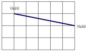
The project involved the realization of various figures and shapes like points, lines, squares, circles, polygons, etc on the VGA screen and the use of optimized version of edge detection and polygon color filling by implementing fencing for which various graphics algorithms were implemented as described below:

Bresenham’s algorithm for line drawing ^[2]

The Bresenham’s line drawing algorithm is an algorithm that determines which points in an n-dimensional pattern should be plotted in order to form a close approximation to a straight line between two given points. It is commonly used to draw lines on a computer screen, as it uses only integer addition, subtraction and bit shifting. It is one of the earliest algorithms developed in the field of computer graphics.

Construction of line segments

Consider a line with initial point (x₁, y₁) and terminal point (x₂, y₂) in device space. Driving Axis is x-axis if the change in x-coordinates is more than the change in y-coordinates or is y-axis if vice-versa. If ∆x = x₂ − x₁ and ∆y = y₂ − y_1, the driving axis (DA) is said to be the x-axis if |∆x| >= |∆y|, and y-axis if |∆y| > |∆x|. The DA is used as the “axis of control” for the algorithm and is the axis of maximum movement. Within the main loop of the algorithm, the coordinate corresponding to the DA is incremented by one unit. The coordinate corresponding to the other axis (usually denoted the passive axis or PA) is only incremented as needed.

Case 1: (x₁, y₁)= and (x₂, y₂) such that |∆x| >= |∆y| and x₁ < x₂, y₁ < y₂

Let the two end points be (x₁, y₁)and (x₂, y₂) such that x₁ < x₂,y₁ < y₂ and |∆x| >= |∆y|. The algorithm begins with the point (x₁, y₁)and illuminates that pixel. Since x is the DA in this example, it then increments the x-coordinate by one. Rather than keeping track of the y coordinate (which increases by m = ∆y/∆x, each time the x increases by one), the algorithm keeps an error bound є at each stage, which represents the negative of the distance from the point where the line exits the pixel to the top edge of the pixel. This value is first set to m − 1, and is incremented by m each time the x-coordinate is incremented by one. If єbecomes greater than zero, we know that the line has moved upwards one pixel, and that we must increment our y coordinate and readjust the error to represent the distance from the top of the new pixel – which is done by subtracting one from є. Here єis initialized to (∆y/∆x – 1) and is incremented by ∆y/∆x at each step. Since both ∆y and ∆x are integer quantities, we can convert to an all integer format by multiplying the operations through by ∆x. That is, we will consider the integer quantity where є_bar is initialized to є_bar = ∆x є = ∆y − ∆x and we will increment є_bar by ∆y at each step, and decrement it by ∆x when є becomes positive.

The integer version of Bresenham’s algorithm is constructed as follows. The (x₁, y₁) and (x₂, y₂) are assumed not equal and integer valued. є_bar is assumed to be integer valued.

∆x = x2 − x1
∆y = y2 − y1
y = y1
єbar = ∆y − ∆x
for x = x1 to x2 − 1
	illuminate (x, y)
	if ( < 0)
	y + = 1
	єbar+ = ∆x
	end if
	x + = 1
	єbar- = ∆y
	next x
finish

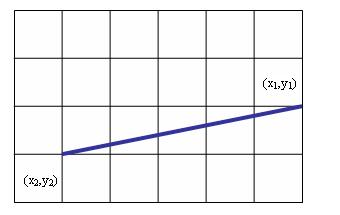
This above algorithm only handles lines that descend to the right.

Case 2: (x₁, y₁) and (x₂, y₂) such that |∆x| >= |∆y| and x₁ > x₂, y₁ < y₂

The same algorithm can be used to plot such a line also. This can be done by swapping (x₁,y₁)and (x₂,y₂ ). The following logic can be included in the algorithm:

if x1 > x2   then
swap(x1, x2)
swap(y1, y2)

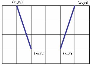
Case 3: (x₁, y₁) and (x₂, y₂) such that |∆y| >= |∆x| and x₁ < x₂, y_{1 <} y₂

The same algorithm can be used to plot such a line also. This can be done by swapping x and y coordinate. That is the line is represented as (y₁, x₁)and (y₂,x₂) to the algorithm. The following logic can be included with the previous algorithm:

if |∆y| >= |∆x| then
swap (x1, y1)
swap (x2, y2)
plot(y,x)

Case 4: (x₁,y₁) and (x₂,y₂) such that |∆x| >= |∆y| and x₁ > x₂, y₁ > y₂

When the value of y coordinate is y₁ > y₂ then y is decremented or when value of y coordinate is y₁<y₂then y is incremented. The following logic can be included to the algorithm:

if  y1 < y2 then
y = y+1
else
y = y-1 

Final Algorithm used to implement lines of different slopes is as follows:

line (x1, y1, x2, y2)
begin
∆x = x2 − x1
∆y = y2 − y1

if |∆y| >= |∆x| then //slopes greater than 45 degrees
swap (x1, y1)
swap (x2, y2)
           end if


if x1 > x2   then 
swap(x1, x2)
swap(y1, y2)
           end if

y = y1
єbar = ∆y − ∆x

for x = x1 to x2 − 1
	if |∆y| >= |∆x| then
		illuminate (y,x) //slopes greater than 45 degrees
	else
illuminate (x, y)
		end if
if (єbar > 0)
y + = 1
єbar+ = ∆x
else 

y - = 1
єbar+ = ∆x
end if
x + = 1
єbar- = ∆y
next x
finish 

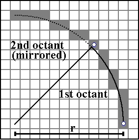
Algorithm for circle drawing ^[2]

The algorithm begins with the general equation of the circle x² + y² = r² which parameterize a circle with radius r and takes only the first octant into consideration. Initially, an arc is drawn which starts at the point (r, 0) and proceeds to the top left in steps, ultimately attaining an angle of 45°. Here, the “fast” direction is the y direction as for the given arc, the change in y direction (upwards) is greater than the change in x direction (left side or negative direction), which is the “slow” direction. Thus, there is always a step in the positive y direction and a step in the negative x direction, every now and then. By dissolving everything into single steps and computing quadratic terms from the previous ones recursively, the frequent computations of squares in the circle equation, trigonometric expressions or square roots can again be avoided.

The equation of the circle given above can be transformed into

0 = x²+y²-r²

where r² is to be computed only single time during initialization. If previous value of x and y are denoted as x_previous and y_previous respectively, we have

x² = (x_previous -1)² = x_preceding² - 2* x_previous +1 
y² = (y_previous -1)² = y_previous² - 2* y_previous +1

Here, the mid point co-ordinates are added when setting a pixel but these frequent integer additions do not limit the performance significantly as square (root) computations are spared in the inner loop.

In the above transformed equation, the zero is replaced by the error term which is derived from an offset of ½ pixel at the start. If P(x, y) represents the current pixel on the graph, then let the error E be how far P is from the correct point on the circle.

Hence, E_now = r² - x² - y².

If E_now ≥ 0, which means that the pixel is either on or inside the circle, a pixel is moved one pixel to the right by x_next = x +1, which makes

Enext= r² − x_next² − y2r² − x_next² − y² = Enow − 2x − 1

Unless an intersection with the perpendicular line takes place, this starting offset leads to an accumulated value of r in the error term. The implementation done for the first octant can be easily extended to other octants by the sign changes for x and/or y and the swapping of x and y, wherever required.

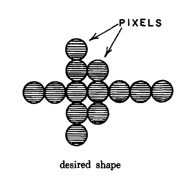
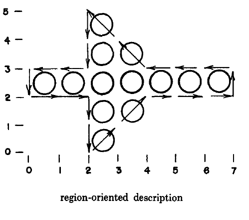
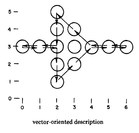
Edge detection and color filling algorithm with fencing ^[3]

For implementing any polygon-filling algorithm, two different raster coordinate systems are possible, region-oriented coordinate system or vector-oriented coordinate system as illustrated in the below figure. In the region-oriented coordinate system, the pixels lie between grid lines and not on the grid lines. This technique is appropriate for applications such as mapping and cartoon animation as polygons sharing a common border will adjoin seamlessly, without sharing any pixels. On the other hand, the vector-oriented coordinate system is one in which pixels lie on grid lines which is appropriate for line-oriented applications such as wiring diagrams.

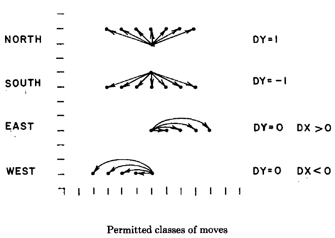
The polygon is represented to the algorithm as a sequence of incremental moves (dx, dy), plus a starting position (x, y), where all values are integers, and these moves describe a closed curve. While the dx values can be any integer, from positive to negative infinity, the dy values can only either be +1, 0, or -1. The algorithm does not consider the null move i.e. (0, 0). There are the following four possibilities or classes of the moves:

North any move in the upwards or positive y direction i.e. dy = 1 is called north regardless of the value of dx.

South any move in the downwards or negative y direction i.e. dy = -1 is called south regardless of the value of dx

East any move in the right or positive x direction i.e. dx > 0 when dy = 0

West any move in the left or negative x direction i.e. dx < 0 when dy = 0

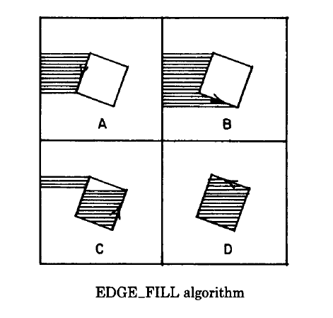
The algorithm used in the project is “Region Edge Fill”. As per this algorithm, at each point where the polygon boundary crosses a scan line, all pixels from that point to the left edge of the screen are inverted. Thus, any point outside the polygon will be inverted an even number of times as shown in the figure. The operation of inverting all pixels to the left of a given X, Y location is denoted as “Clear”. The only moves which cause clearing are north and south moves, since east and west moves do not intersect scan lines. When such a move is made, the pixel nearest the intersection point (halfway between grid lines) is the pixel from which clearing is done.

The algorithms are written as though the moves were being read from a sequential file. This simplifies the presentation and emphasizes the finite-memory nature of the algorithm as given below.

PROCEDURE region_edge_fill;
    VAR x, y, dx, dy, i: INTEGER;
    PROCEDURE invert_scan_segment(xl, x2, y: INTEGER); BEGIN
        IF xl < x2 THEN
            FOR i := xl + 1 TO x2 DO invert_pixel(i, y)
        ELSE
            FOR i := x2 + 1 TO xl DO invert_pixel(i, y);
        END;
    PROCEDURE clear(x, y: INTEGER); BEGIN
        invert_scan_segment(0, x, y);
        END;
    BEGIN                                             {begin REGION_EDGE_FILL}
        read(x, y);                                   {read starting position}
                                                      {for each move}
        WHILE not end_of_file DO BEGIN
            read(dx, dy);                             {read the move}
CASE Class (dx, dy) OF                                {do the appropriate clear}
              east: Nop;
              north: clear(x + trunc(dx/2), y);
              west: Nop;
              south: clear(x + trunc(dx/2), y - 1);
              END;
x := x + dx;                                          {do the move}
y := y + dy;
END;                                                  {end REGION_EDGE_FILL}