
Hardware Design
Control Logic
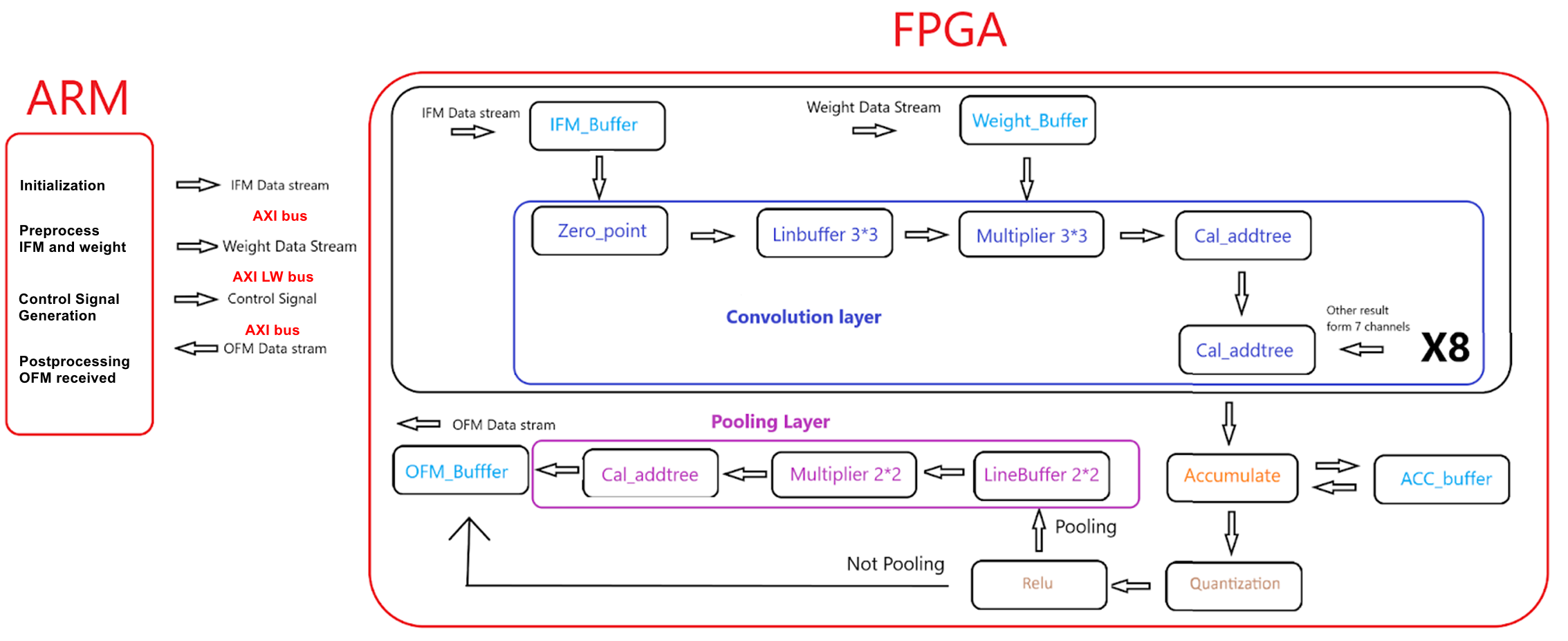
Each complete convolution layer encompasses five sequential stages, initiated by the ARM core providing input channel information and relative parameters, culminating in the output result being sent back to the ARM core: RECV, LOAD, CALC, WRITE, and SEND.
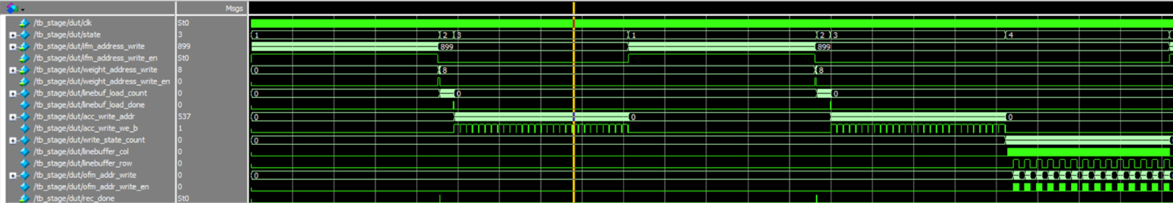
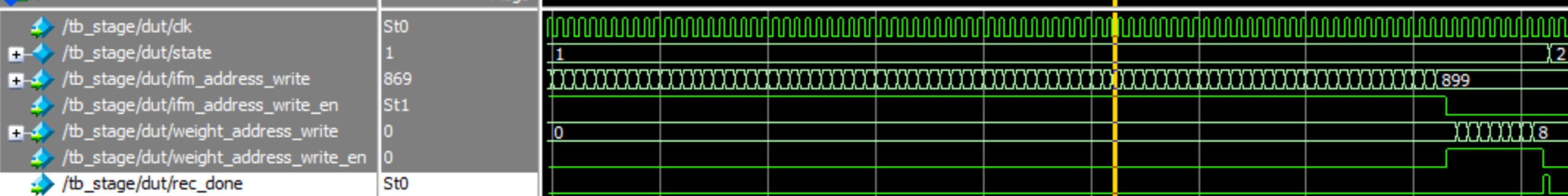
The figure illustrates the overall Modelsim simulation. In this test bench, we set the input channels to 16, meaning the conversion layer will repeat once since it can process 8 channels simultaneously. As indicated by the state variable, the process starts at RECV (Stage 1), moves to LOAD (Stage 2), and then to CALC (Stage 3). Due to the 16 input channels, the conversion stages are repeated. Finally, the process enters WRITE (Stage 4), where all the data is written into the ofm_Buffer.
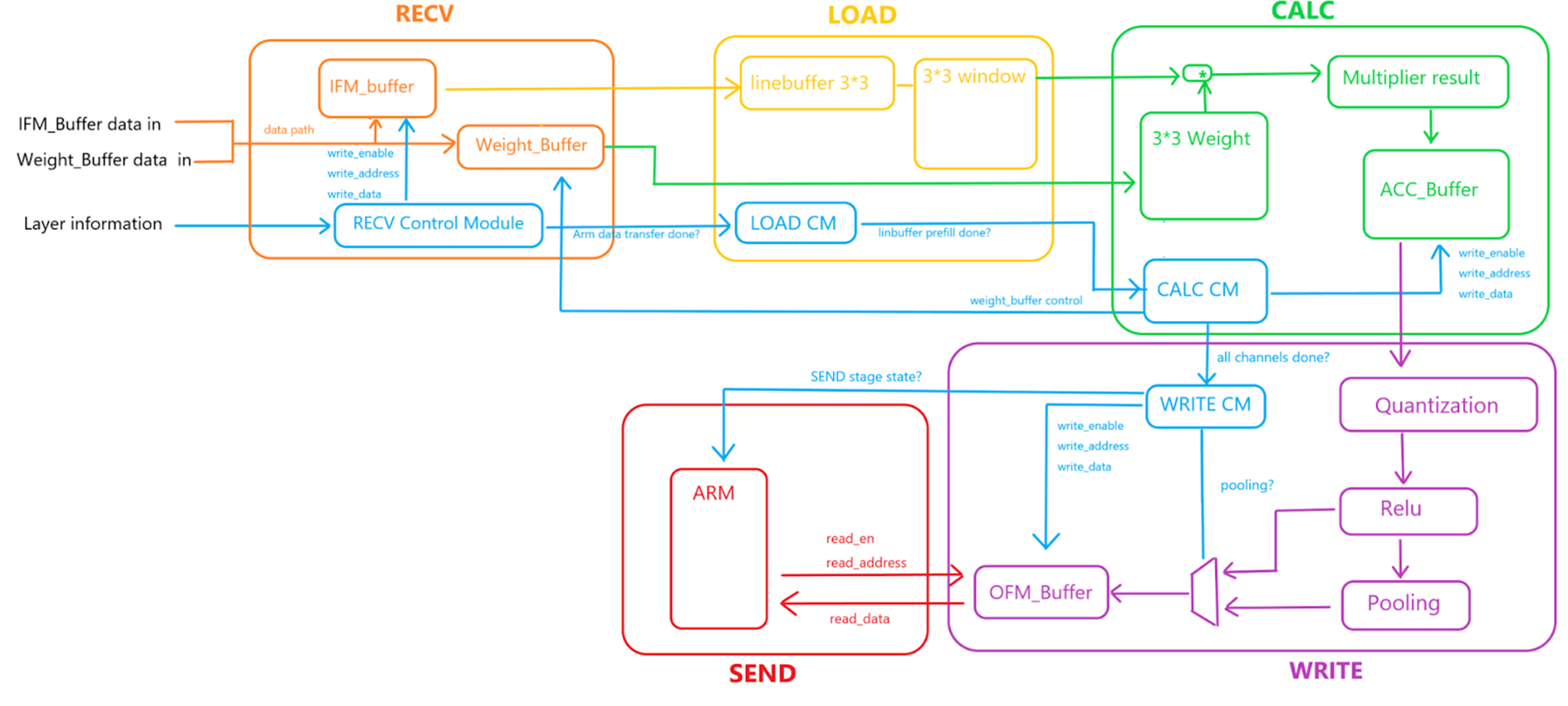
RECV
- Receive the Input Feature Map (IFM) and weight data stream from the ARM core via the AXI channel.
- Store the data and weights in the IFM_Buffer and Weight_Buffer.
- Since we only have one 64-bit data path, the RECV control module will perform the IFM_Buffer write first, then perform the Weight_Buffer after. We have an input signal from the arm to tell the RECV control module if we are currently writing the data for the IFM_Buffer or the Weight_Buffer.
- The write_enable, write_address, and write_data come from the ARM core directly.
Modelsim (Stage 1): During this stage, the testbench continuously writes data into the ifm_buffer, causing the ifm_address_write to increment until it reaches 899, indicating that all ifm data has been written to the ifm_buffer. Following this, the weight data is written into the weight buffer. As shown in the waveform, the weight_address_write starts counting after the ifm_address_write reaches 899. The stage transitions upon receiving the rec_done signal from the testbench.
LOAD
- Preload the data into the Linbuffer 3*3 and transfer it to the next stage once the Linbuffer warms up and produces the correct 3*3 window output.
- Because the linbuffer works as a data stream, the LOAD control module will not be doing any interference for the datapath. It only tells if the current 3 *3 window is valid data and moves to the next stage based on the buffer counter.
Modelsim (Stage 2): When the linebuf_load_done signal is set to high, it indicates that the window buffer is ready for the conversion layer input. Consequently, the linebuffer_load_count increments to 65, accounting for both the buffer warm-up time and the pipeline conversion delay. The total time taken is calculated as Time_taken = size_fm_in * 2 + 3.

CALC
- Execute convolution calculations. Temporarily store the current 8 channels' convolution results in the ACC_buffer.
- Check if all input channels are processed; if so, proceed to the WRITE stage; otherwise, return to the RECV stage to receive the next 8 input channels.
- CALC control module gives a control signal to the ACC_Buffer about write_enable, write_address, and write_data based on this internal counter.
Modelsim (Stage 3): After a few cycles of delay due to the conversion operation, data is written into the acc_buffer. However, the output data from the conversion layer becomes invalid for two cycles every 28 cycles because each row contains 28 data points. The reason for this invalidation is explained in the linebuffer 3x3 section below.

WRITE
- Determine whether pooling is required for this layer. If so, perform the pooling operation; otherwise, write the data directly into the OFM_Buffer.
- Pooling operation also necessitates a 2*2line buffer, requiring wait time until the line buffer is warmed up and can produce the correct 2*2 windows.
- Once the pooling operation is completed, write the data back to the OFM_Buffer.
- The data path for Quantization, Relu, and pooling is not controlled by the WRITE control module, it works like a pipeline there always have data flow inside.
- The WRITE control module is responsible for telling the FPGA if we want to perform pooling and when is all the correct data being written into the OFM_Buffer.
Modelsim (Stage 4): At the beginning of this stage, all input channels are performing calculations, and data is being written into the acc_buffer. After a few cycles of delay in the write_state_count for the pipeline, including the quantization and ReLU layers, we start writing data into the ofm_buffer. Similar to the linebuffer 3x3, during the pooling operation, the output of the 2x2 window buffer becomes invalid when filling the next 2x2 window. This is why we use linbuffer_row and linbuffer_col to keep track of the linebuffer's position.

SEND
- Transmit the data back to the ARM core. Upon completion of this operation, one complete convolution layer is finished.
- Reset to the RECV stage to process information from the next layer.
Linebuffer 3*3 convolution
Why is a Linbuffer 3*3?
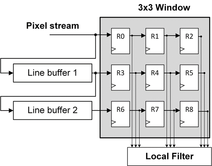
A 3x3 window line buffer in image processing temporarily stores three rows of pixel data to provide efficient access to a 3x3 neighborhood around each pixel. It uses two line buffers to hold the last two rows and shift registers to handle the current row. As each pixel is processed, the window shifts right by updating the shift registers with the next pixel in the row. Once a row is fully processed, the line buffers update to include the next row, maintaining the 3x3 window until the entire image is processed. This setup is crucial for operations like convolutional filtering and feature detection.
How does the Control Logic work?
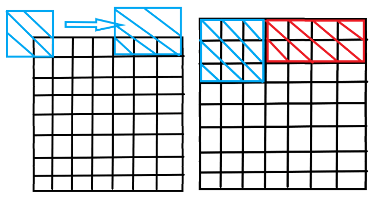
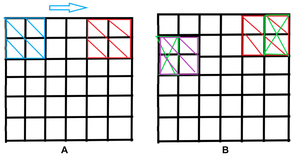
In Figure 13 left, we have an image with dimensions 7x8 pixels and a window size of 3x3. The left window illustrates how the first data is loaded into the line buffer, while the right window shows how the last bit of data is written into the line buffer. At this stage, since the buffer is not yet filled with image data, the output from the window buffer is not valid.
In Figure 13 right, we continue to fill the line buffer until it is completely filled. At this point, it takes 2 * row_size + 3 cycles to fill the line buffer. Now, the window buffer is valid and ready to output data to the next conversion layer.
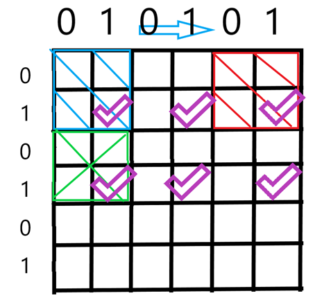
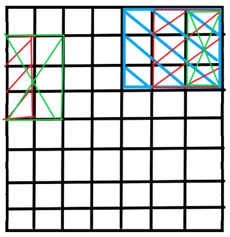
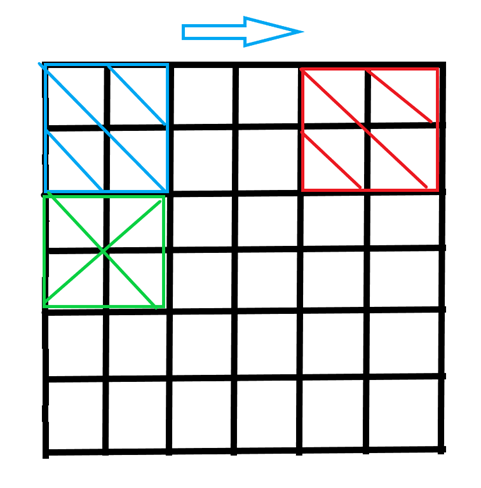
However, after the line buffer is filled, what happens when we reach the end of each row? Will the window buffer remain valid in the subsequent cycles? As shown in Figure 14, the data inside the blue window remains valid. However, as we continue to insert data into the line buffer, the window buffer becomes invalid for the next two cycles, represented by the red and green boxes. This example demonstrates that after loading data into the buffer, the window buffer becomes invalid when we reach the end of each row. This can be calculated as follows:
If linbuffer_countof is not a multiple of row_size and its next cycle, the line buffer output is considered valid.
Linebuffer 2*2 Max polling
Max polling operates on a 2x2 grid of values within a feature map and selects the maximum value from that grid. This process reduces the spatial dimensions of the input, helping to downsample the data and make the model more computationally efficient while retaining important features.
The 2x2 line buffer operates similarly to the 3x3 line buffer, but instead of outputting a valid window buffer for the conversion operation, it moves the blue 2x2 window to the right, reaching the position of the red window, as shown in Figure 15(a). With the step set to two and the buffer capturing one data element per clock cycle, it takes two cycles to produce the next valid output. After completing a valid row of 2x2 window outputs, the data in the next row, which was written into the line buffer, becomes invalid, as illustrated in Figure 15(b).
In Figure 16, the window buffer must wait for the next two rows of data to be completely written into the buffer before it can output valid data. As shown, the green window indicates when the data will become valid again after the red window.
To address this issue and control when the window buffer becomes valid, we can implement two counters: row_counter and column_counter. These counters will initiate simultaneously once the line buffer is fully loaded. The column_counter will cyclically count between 0 and 1. Meanwhile, the row_counter will switch these values after completing one row of data. As depicted in Figure 17, the window buffer will only output valid data when both the row_counter and column_counter reach 1 simultaneously.