Synthesizing Birdsong
ECE 4760, Fall 2021, Adams/Land
Webpage table of contents
Background and Introduction
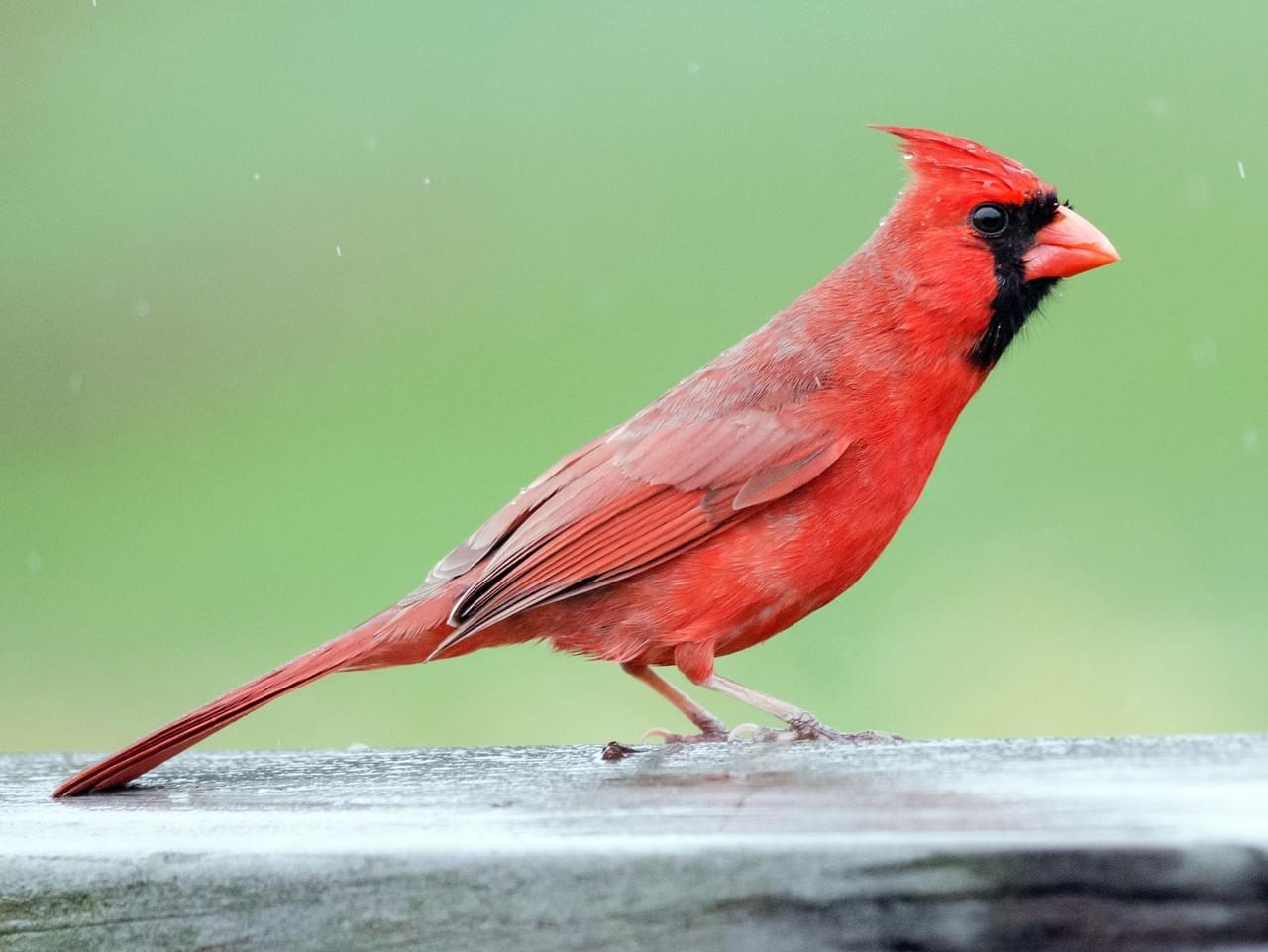
We will be using direct digital synthesis to generate the call of the northern cardinal. Specifically, this adult male northern cardinal recorded by Gerrit Vyn in 2006. This bird was recorded in Texas, but cardinals are also common in Ithaca and throughout the eastern United States. If you pay attention when you're walking through campus, you may hear one singing. The males are a very striking red. You can read more about the cardinal here.
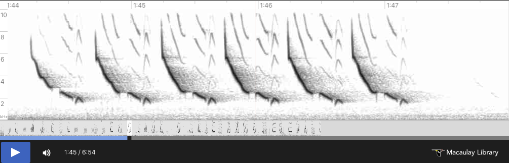
Cardinals have a variety of songs and calls. We will be synthesizing on of its most common songs, which you can hear in the first ten seconds of the recording below:
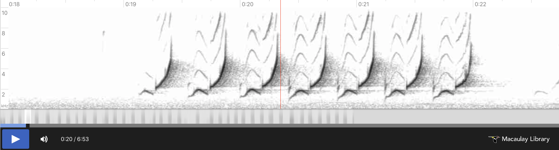
Here is a screenshot of the spectrogram for the song that we'll be synthesizing. Cardinals and many other songbirds produce almost pure frequency-modulated tones. As can be seen in the spectrogram below, the cardinal sweeps through frequencies from ~2kHz to ~7kHz. We'll assume that the dominant tones (the darkest lines on the spectrogram) are significantly louder than all other frequencies (the lighter lines). We'll only synthesize these loudest frequencies. The generated song sounds quite realistic under this assumption. Your synthesizer will be controlled via a keypad.
Deconstructing the song
This song can be decomposed into three sound primitives: a low-frequency swoop at the beginning of each call, a chirp after each swoop which moves rapidly from low frequency to high frequency, and silence which separates each swoop/chirp combination. We will synthesize each of these primitives separately, and then compose them to reconstruct the song.
Swoop
Swoop Analysis
By pasting the above spectrogram in Keynote or PowerPoint and drawing lines on it, you can determine that the length of the chirp is approximately 130 ms. Since the DAC gathers audio samples at 44kHz, this means that the chirp lasts for $0.130\text{sec} \cdot \frac{44000\text{ samples}}{1\text{ sec}} = 5720\text{ samples}$. We'll approximate the frequency curve by sine wave of the form:
where $y$ is the frequency in Hz, and $x$ is the number of audio samples since the chirp began. Since the swoop starts and ends at 1.74kHz and peaks at 2kHz, we can setup the following system of equations to solve for the unknown parameters $k$, $b$, and $m$:
From which we can find $b=1740$, $k = -260$, $m = \frac{-\pi}{5720}$. So, the equation is given by:
Plot the simulated swoop of frequencies:
plt.plot(-260*numpy.sin(-numpy.pi/5720*numpy.arange(5720)) + 1740)
plt.xlabel('Audio samples'); plt.ylabel('Hz'); plt.title('Swoop frequencies')
plt.show()

Swoop Simulation
Some DDS parameters, including the sample rate (44kHz), a 256-entry sine table, and the constant $2^{32}$:
Fs = 44000 #audio sample rate
sintable = numpy.sin(numpy.linspace(0, 2*numpy.pi, 256))# sine table for DDS
two32 = 2**32 #2^32
And now we can synthesize audio samples.
swoop = list(numpy.zeros(5720)) # a 5720-length array (130ms @ 44kHz) that will hold swoop audio samples
DDS_phase = 0 # current phase
for i in range(len(swoop)):
    frequency = -260.*numpy.sin((-numpy.pi/5720)*i) + 1740 # calculate frequency
    DDS_increment = frequency*two32/Fs # update DDS increment
    DDS_phase += DDS_increment # update DDS phase by increment
    DDS_phase = DDS_phase % (two32 - 1) # need to simulate overflow in python, not necessary in C
    swoop[i] = sintable[int(DDS_phase/(2**24))] # can just shift in C
In order to avoid non-natural clicks, we must ramp the amplitude smoothly from 0 to its max amplitude, and then ramp it down. We'll do this by multiplying the chirp by the linear ramp function shown below:
# Amplitude modulate with a linear envelope to avoid clicks
amplitudes = list(numpy.ones(len(swoop)))
amplitudes[0:1000] = list(numpy.linspace(0,1,len(amplitudes[0:1000])))
amplitudes[-1000:] = list(numpy.linspace(0,1,len(amplitudes[-1000:]))[::-1])
amplitudes = numpy.array(amplitudes)
plt.plot(amplitudes);plt.title('Amplitude envelope');plt.show()

# Finish with the swoop
swoop = swoop*amplitudes

Here is what the swoop looks like:
plt.plot(swoop);plt.title('Amplitude-modulated swoop');plt.show()

And here is what it sounds like:
Audio(swoop, rate=48000)
Chirp
Chirp Analysis
By pasting the above spectrogram in Keynote and drawing lines on it, you can determine that the length of the chirp is also approximately 130 ms (5720 samples). We'll approximate the frequency curve by a quadratic equation of the form:
where $y$ is the frequency in Hz, and $x$ is the number of audio samples since the chirp began. Since the chirp starts at 2kHz and ends at 7kHz, we can setup the following system of equations to solve for the unknown parameters $k$ and $b$:
This is two equations with two unknowns. Solving, we find that $b=2000$ and $k\approx 1.53 \times 10^{-4}$. So the quadratic equation for the chirp is:
Plot the simulated chirp frequency sweep:
plt.plot(1.53e-4 * numpy.arange(5720)**2. + 2000);plt.title('Chirp frequencies');plt.show()

Chirp Simulation
And now we can synthesize audio samples.
chirp = list(numpy.zeros(5720)) # a 5720-length array (130ms @ 44kHz) that will hold chirp audio samples
DDS_phase = 0 # current phase
for i in range(len(chirp)):
    frequency = (1.53e-4)*(i**2.) + 2000 # update DDS frequency
    DDS_increment = frequency*two32/Fs # update DDS increment
    DDS_phase += DDS_increment # update DDS phase
    DDS_phase = DDS_phase % (two32 - 1) # need to simulate overflow in python, not necessary in C
    chirp[i] = sintable[int(DDS_phase/(2**24))] # can just shift in C
In order to avoid non-natural clicks, we must ramp the amplitude smoothly from 0 to its max amplitude, and then ramp it down. We'll do this by multiplying the chirp by the linear ramp function shown below:
# Amplitude modulate with a linear envelope to avoid clicks
amplitudes = list(numpy.ones(len(chirp)))
amplitudes[0:1000] = list(numpy.linspace(0,1,len(amplitudes[0:1000])))
amplitudes[-1000:] = list(numpy.linspace(0,1,len(amplitudes[-1000:]))[::-1])
amplitudes = numpy.array(amplitudes)

# Finish with the chirp
chirp = chirp*amplitudes
The entire amplitude-modulated chirp looks like this:
plt.plot(chirp);plt.title('Amplitude-modulated chirp');plt.show()

And it sounds like this:
Audio(chirp, rate=44000)
Silence
The amount of time between swoop/chirps is also (approximately) 130ms or 5720 cycles.
silence = numpy.zeros(5720)
Assembling the song
We assemble the song by playing the swoop/chirp/silence in succession:
song = []
for i in range(5):
    song.extend(list(swoop))
    song.extend(list(chirp))
    song.extend(list(silence))
song.extend(list(swoop))
song.extend(list(chirp))
song.extend(list(silence))
song = numpy.array(song)
plt.plot(song);plt.title('Full song');plt.show()

Listen to it:
Audio(song, rate=44000)
And view the spectrogram of the Python-generated song:
f, t, Sxx = signal.spectrogram(song, Fs)
plt.pcolormesh(t, f, Sxx,  shading='gouraud')
plt.ylabel('Hz'); plt.xlabel('Time (sec)')
plt.title('Spectrogram of Python-generated birdsong')
plt.ylim([0,10000])
plt.show()

Hardware
The Big Board which you will be using features a port expander, DAC, TFT header-socket, programming header-plug, and power supply. See the construction page for specific code examples of each device on the big board. The connections from the PIC32 to the various peripherals is determined by the construction of the board. The list is repeated here.
PIC32 i/o pins used on the big board, sorted by port number
Any pin can be recovered for general use by unplugging the device that uses the pin (of course, if you're doing this lab remotely, you will not be able to unplug these devices). SPI chip select ports have jumpers to unplug.
RA0 on-board LED. Active high.
RA1 Uart2 RX signal, if serial is turned on in protothreads 1_2_2
RA2 port expander intZ
RA3 port expander intY
RA4 PortExpander SPI MISO
-----
RB0 TFT D/C
RB1 TFT-LCD SPI chip select (can be disconnected/changed)
RB2 TFT reset
RB4 DAC SPI chip select (can be disconnected/changed)
RB5 DAC/PortExpander SPI MOSI
RB6 !!! Does not exist on this package!!! (silk screen should read Vbus)
RB9 Port Expander SPI chip select (can be disconnected/changed)
RB10 Uart2 TX signal, if serial is turned on in protothreads 1_2_2
RB11 TFT SPI MOSI
RB12 !!! Does not exist on this package!!! (silk screen should read Vusb3.3)
RB14 TFT SPI Sclock
RB15 DAC/PortExpander SPI Sclock
But note the few silk-screen errors on the board.
SECABB version 2 silk screen errors. (fixed on version 2.1)
- Edge connector pin marked RB6 -- RB6 does not exist on this package! Silk screen should read Vusb.
- Edge connector marked RB12 -- RB12 does not exist on this package! Silk screen should read Vusb3.3
- LED D1 outline -- Silk screen should have flat side should be oriented toward PIC32
Software
Software you will use is freely downloadable and consists of:
(All of this is already installed on the lab PC's). More information can be found at the links below.
- Getting started with PIC32
- MPLABX IDE users guide
- 32 bit peripherals library -- PLIB examples
- 32 bit language tools and libraries including C libraries, DSB, and debugging tools
- XC32 Compiler Users Guide
- PIC32MX2xx datasheet -- Errata
- MicrostickII pinout
- PIC32MX250 configuration options
- JTAG enable overrides pins 13, 14, and 15
- Primary oscillator enable overrides pins 9 and 10
- Secondary oscillator enable overrides pins 11 and 12
- PIC32 reference manual
- This is huge, better to go to the PIC32 page then Documentation --> Reference Manual and choose the section
- Specific pages from the PIC32 datasheet
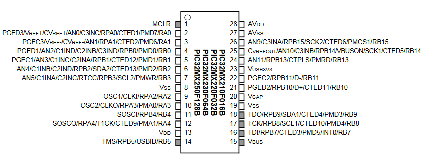
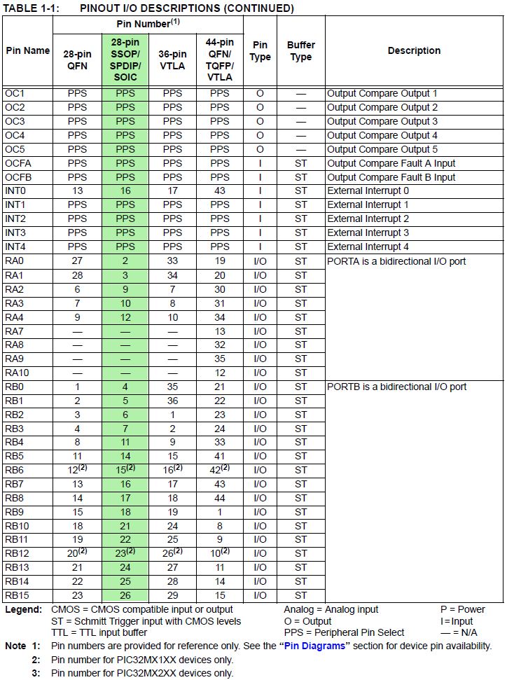
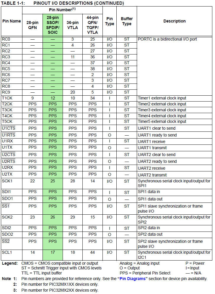
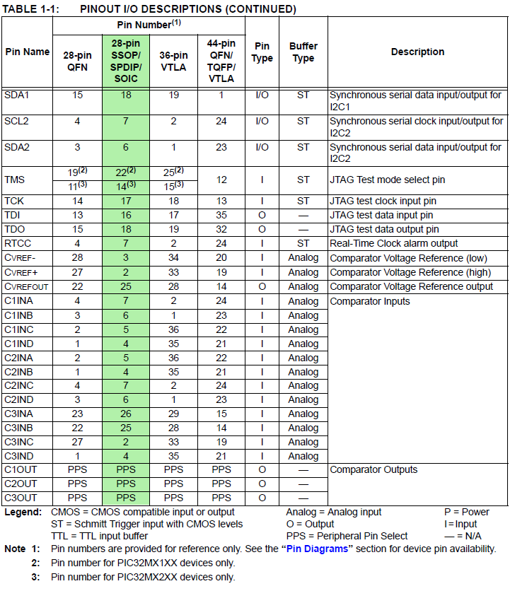
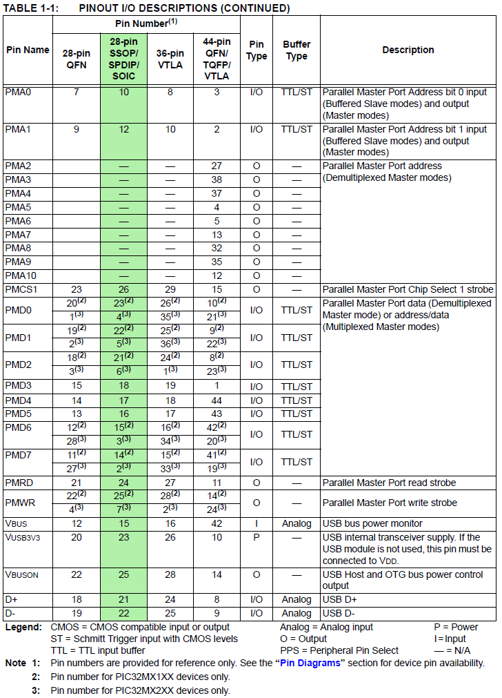
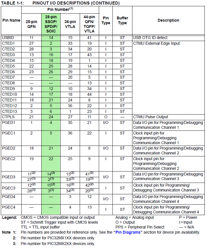
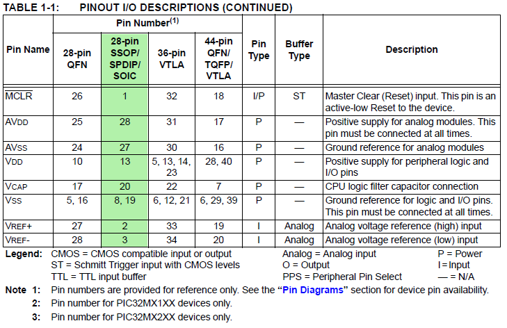
- PIC32MX250F128B PDIP pinout by pin
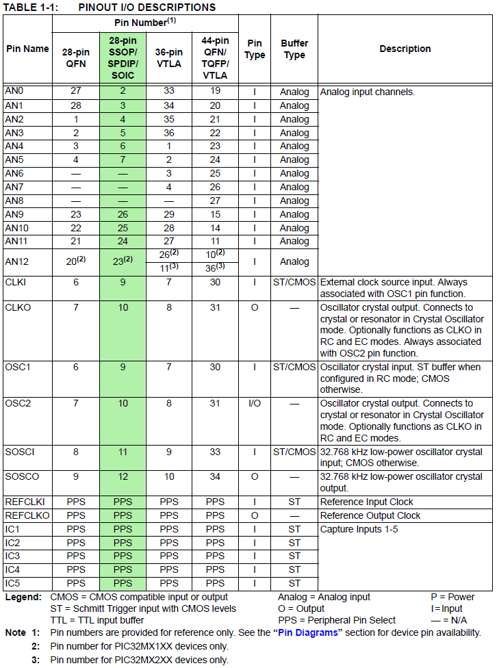
- PIC32MX250F128B:: Signal Names $\rightarrow$ Pins::1, 2, 3, 4, 5, 6, 7 PDIP highlighted in green (for PPS see next tables)
- PIC32MX250F128B Peripheral Pin Select (PPS) input table
- Example: UART receive pin ::: specify PPS group, signal, logical pin name
PPSInput(2, U2RX, RPB11);
// Assign U2RX to pin RPB11 - Physical pin 22 on 28 PDIP
- Example: UART receive pin ::: specify PPS group, signal, logical pin name
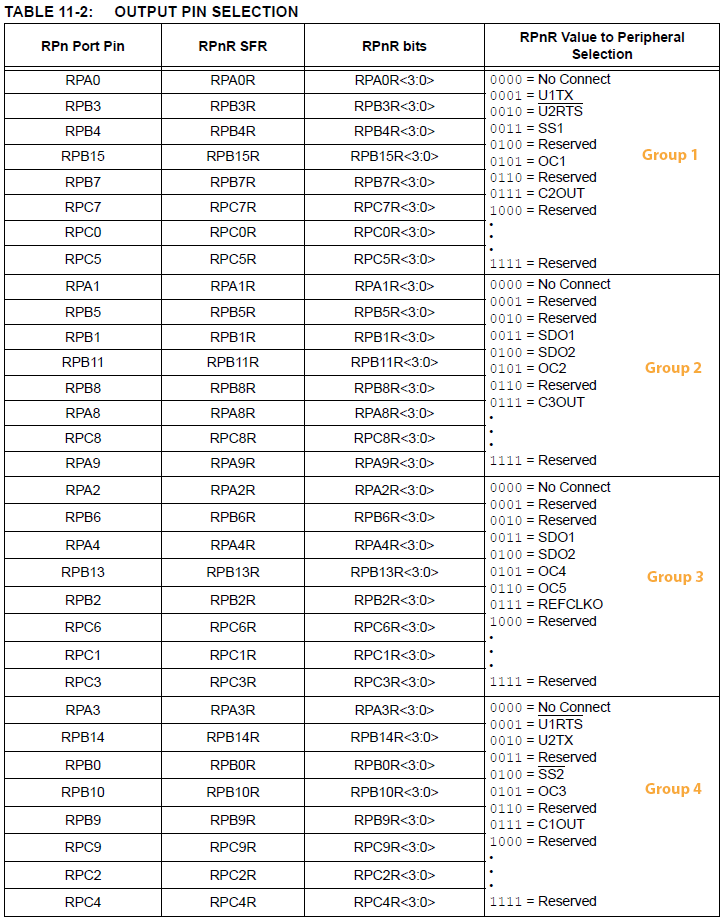
- PIC32MX250F128B Peripheral Pin Select (PPS) output table
- Example: UART transmit pin ::: specify PPS group, logical pin name, signal
PPSOutput(4, RPB10, U2TX);
// Assign U2TX to pin RPB10 - Physical pin 21 on 28 PDIP
- Example: UART transmit pin ::: specify PPS group, logical pin name, signal
Oscilloscope software:
- See this webpage
Programmer
PicKit3
Here is the pinout for the PICKIT3, the programmer which was used to develop the boards you will be using. On both the big and small boards, J1 marks pin1 of the 6-pin ICSP header.
| Signal | PICkit3 (ICSP) connector on board |
|---|---|
| MCLR | 1 |
| ground | 3 |
| prog data (PGD) | 4 |
| prog clock (PGC) | 5 |
Procedure
- The current version of Protothreads is 1_3_2. All example programs using this threader may be found on the Development board page. Download the ZIP file on this page to get all the libraries and substitute in the following source code:
Program example 3, DDS_Accum_Expander_BRL4.c on the Development board page is the basis for this lab. - For an example of controlling the PIC from a Python interface, see the remote learning page
- For most of the semester you will be using the TFT LCD for output and debugging. You will need to use some of the graphics library calls described in the test code in this lab.
Test code: TFT_test_BRL4.c -- displays color patches, system time, moves a ball, generates a slow ramp on the DAC, and blinks the LED - You may want to refer to the ProtoThreads page for the general threading setup.
- Timing of all functions in this lab, and every exercise in this course will be handled by interrupt-driven counters, (including the builtin functions in ProtoThreads) and not by software wait-loops. This will be enforced because wait-loops are hard to debug and tend to limit multitasking. You may not use any form of a delay(mSec) function.
- The oscilloscope is essential for debugging this lab (and every lab). The oscilloscope is the only way of deciding if -- It doesn't work! -- results from hardware or software.
Relevant resources
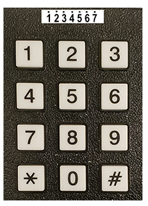
Keypad
Your birdsong synthesizer will be cotrolled via a keypad. Please see this page for examples of and information about the the keypad that we will be using.
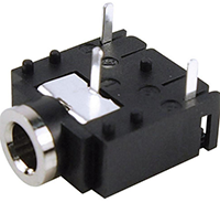
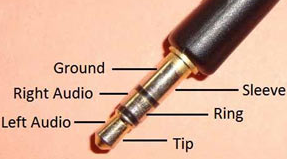
DAC and audio output
The SPI DAC you will use is the MCP4822. The DAC analog output is marked DACA or DACB on the SECABB. The SPI connections are supplied on the Big Board (SECABB), as long as you connect the DAC_CS jumper. Section 5.1 and 5.2 of the MCP4822 datasheet discussed the way the the DAC uses SPI. The edge connector pin marked DACA or DACB will go (optionally through a low pass filter) to an audio socket, to be connected to the green audio plug of the speakers. If you are going to design a lowpass filter for the DAC, then you need to know that the input impedance of the speakers is around 10 Kohm.
Sound synthesis
Generally speaking you want to make pleasant sounding synthesis. You may want to look at the sound synthesis page. I suggest starting with a linear attack of about 1000 samples, a decay of about 1000 samples, and a sustain as long as necessary for a 130ms chirp/swoop.
Program Organization and Debugging
Program Organization
I suggest that you organize the program as follows. If a different organization makes more sense to you, that's ok. This is just a suggestion.
- Protothreads maintains the ISR-driven, millisecond-scale timing as part of the supplied system. Use this for all low-precision timing (can have several milliseconds jitter).
- Synthesis ISR uses a timer interrupt to ensure an exact 44KHz synthesis sample rate.
- DDS of sine waves
- DAC output
- Sample count for precise timing of sounds
- Main sets up peripherals and protothreads then just schedules tasks, round-robin
- Keypad Thread
- Scans and debounces the keypad and any other buttons you may use
- Your state machine must debounce all 12 keys.
- Parses the command (if any) and updates state variables (play mode, sound list, etc.)
- Waits for 10-30 mSec using
PT_YIELD_TIME_msec(time), then repeats.
- Play Thread
- Waits to be semaphore-signalled by a different thread
- Plays the sound associated with each button press recorded in the global array by setting up the DDS parameters associated with each sound
- Maintains playback timing using the sample count from the timer ISR
You may find some previous year's lectures useful. You may also find Bruce's lectures useful.
Debugging
If your program just sits there and does nothing:
- Did you turn on interrupts? The thread timer depends on an interrupt.
- Did you write each thread to include at least one
YIELD(orYIELD_UNTIL, orYIELD_TIME_msec) in thewhile(1)loop? - Did you schedule the threads?
- Did you ask to initialize the TFT display in the code, while not having a TFT on the board?
- Does the board have power?
If your program reboots about 5 times/second:
- Did you exit from any scheduled threads? This blows out the stack.
- Did you turn on any interrupt source and fail to write an ISR for that source?
- Did you divide by zero? A divide by zero is an untrapped exception.
- Did you write to any non-existant memory location, perhaps by using a negative (or very large) array index?
If your thread state variables seem to change on their own:
- Did you define any automatic local variable? Local variables in a thread should be static.
- Are your global or static arrays big enough to clobber the stack in high memory? You should be able to use over 30kbytes.
Weekly Checkpoints and Lab Report
Note that these checkpoints are cumulative. In week 2, for example, you must have also completed all of the requirements from week 1.
Week one required checkpoint
By the end of lab session in week one you must have either built and tested your own board or tested a prebuilt board.
- Before you test, be sure to attach the chip-select jumpers for the Port Expander, TFT, and DAC.
- You may find last year's Day Zero webpage helpful. You can ignore the sections on establishing a remote desktop connection, since we'll be conducting our labs in person this semester.
- Testing includes TFT, DAC, LED, and the i/o expander with Keypad. You can omit the serial test for this lab. See the Development Board page.
Week two required checkpoint
- Basic keypad interface working. You should be able to press 1 on the keypad and hear exactly one swoop sound (not necessarily amplitude modulated) and you should be able to press 2 on the keypad and hear exactly one chirp sound.
- Both sounds should appear on the scope.
- Do this by integrating the DDS_Accum_Expander_BRL4.c on the Development board page and example on the keypad page
- Finishing a checkpoint does NOT mean you can leave lab early!
Week three assignment
Timing of all functions in this lab, and in every exercise in this course will be handled by interrupt-driven counters, not by software wait-loops. ProtoThreads maintains an ISR driven timer for you. This will be enforced because wait-loops are hard to debug and tend to limit multitasking
Write a Protothreads C program which will:
- The program starts in play mode. The program will play the swoop sound when the 1 key is pressed and the chirp sound when the 2 key key is pressed. Each sound will play for 130ms, exactly once, independent of the duration of the button push.
- The program will produce 130ms of silence when the 3 key is pressed. This is mostly useful in record mode (see below).
- In play mode, the program will play the recorded sequence of sounds. The sounds will play with an amplitude envelope that you choose. There may not be any clicks, pops, or other audio artifacts.
- The program should have two modes:
- Upon power-up or reset the system should go into play mode and play a sound for each button press (swoop for key 1, chirp for key 2, and 130 ms of silence for key 3).
- Pressing and holding a separate button (not the keypad) or toggling a switch puts the system into record mode so that each button press is recorded for later playback. Recording continues until the record mode toggle is released. The duration of each button press does not affect the recording.
- The program should include two frequency sweeps (the swoop and chirp) that you can hard-code.
- There should be no clicks, pops, or other audio facts of synthesis.
When you demonstrate the program to a staff member, you will be asked to play back a sequence of sounds which simulates the birdsong above, and to play back a random sequence of swoops/chirps/silences. At no time during the demo can you reset or reprogram the MCU.
ECE 5730 students
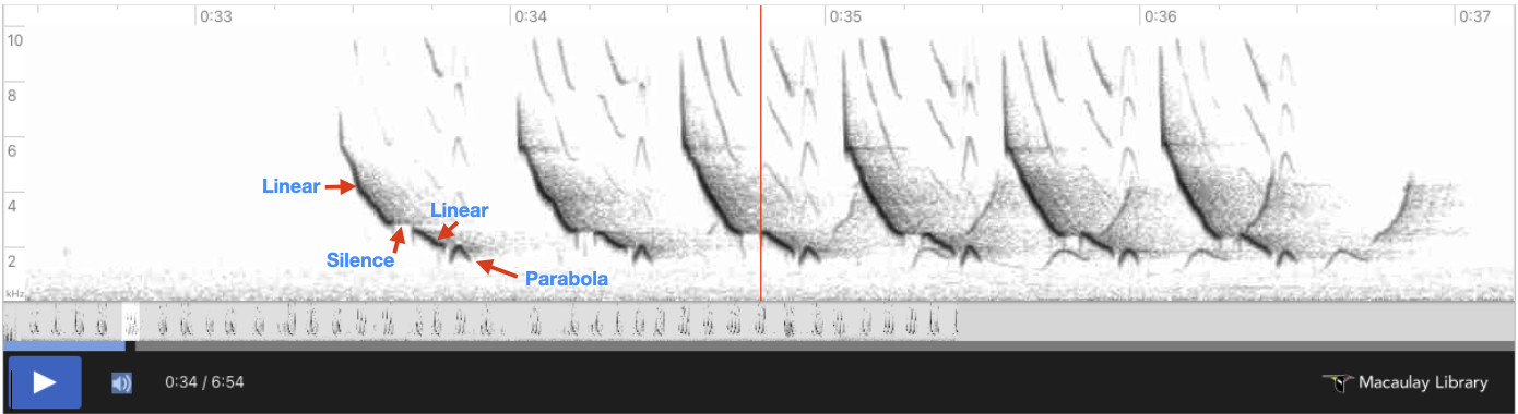
In addition to the above, ECE 5730 students should synthesize another Northern Cardinal song, shown below. You may deconstruct this song into 4 sound primitives, as illustrated below. Fit these frequency sweeps to functions using similar analysis to that shown at the top of this document.
Each of these 4 sound primitives should be mapped to 4 additional keys on the keypad.
You may fit to any function that you like. 2 linear functions and a parabolic function sound nice.
You can also synthesize songs for other, more challenging birds like the Baltimore oriole. (If you're lucky, you can spot these in Ithaca too. They're gorgeous and have a very distinctive song).
Lab report
Your written lab report should include the sections mentioned in the policy page, and:
- A scope display of a swoop/chirp birdcall showing rise, sustain, fall
- A spectrogram of the sound produced by your MCU
- A heavily commented listing of your code
Demonstrations of working system
By plugging the Pic into the microphone input of the PC, we can record the sound that it generates and create a spectrogram of the Pic-generated birdsong:
samplerate, data = wavfile.read('./Bird.wav')
frequencies, times, spectrogram = signal.spectrogram((data[80000:191000,0]+data[80000:191000,1])/2., samplerate)
plt.pcolormesh(times, frequencies, spectrogram,  shading='gouraud')
plt.ylabel('Hz'); plt.xlabel('Time (sec)')
plt.title('Spectrogram of PIC-generated birdsong')
plt.ylim([0,10000])
plt.show()

Includes (please ignore)
import numpy
import matplotlib.pyplot as plt
from IPython.display import Audio
from IPython.display import Image
from scipy import signal
from scipy.fft import fftshift
from scipy.io import wavfile
plt.rcParams['figure.figsize'] = [12, 4]
from IPython.core.display import HTML
HTML("""
<style>
.output_png {
    display: table-cell;
    text-align: center;
    vertical-align: middle;
}
</style>
""")