2. (Due Tues Feb 5)

1. Consider an infinte cable modeled as an infinite ladder of resistors as shown in section. Derive the input resistance. Do this by computing the equlivalent input resistance of the infinite ladder of resistors, then taking the limit as the ladder step size becomes zero.
2. The lecturer stated that concentrations of ions inside and outside the cell don't change as the cell charges to Nernst equlibirum from zero voltage. Using the concentrations of ions given in lecture, justify this statement for a spherical cell. Assume a cell diameter of 20 micrometers, a resting potential of -70 millivolts and a membrane capacitance of 1 microfarad/cm².
3. Using HHsim, answer the questions in sections III, IV and V of the HHsim exercises page.

3. (Due Tues Feb 12)

1. Using HHsim, answer the questions in section VI of the HHsim exercises page.
2. Using HHsim and using long stimulus pulses, plot action potential frequency versus current strength using the longest stimulus pulse you can make (40 mSec). Is the rate linear with current strength in any region above threshold? Why does the rate max out? Why does the action potential amplitude drop at higher frequencies? Explain in terms of gate recovery times.
3. Using HHsim investigate what happens near threshold. Use a long pulse (40 mSec). You may need to vary the current strength by as little as 0.001 to find a threshold. Do you see oscillations? Substandard action potential amplitudes?
4. For the resting potential equivalent circuit given in section, compute the resting potential. Does it match the ion dependencies in the Goldman equation?

4. (Due Tues Feb 26)

Read the details of the Hodgkin-Huxley model. Down load this ZIP file which contains a simple Hodgkin Huxley simulator called HHpgm1.m and a few required functions.

1. Modify the program so that the current injection list can be of arbitrary length. This will include changing the plotting commands so that the resulting graphs are arranged in a reasonable fashion. Print a few examples.

2. Add the ability to compute the firing frequency of the model cell for each of the stimuli presented and to plot the current amplitude versus frequency in a separate figure window. Print the resulting curve.

3. Modify the program so that there are two independent HH cells, each of which has a steady current input, as well as synaptic input from the other cell. The plots should be modified to show one cell in red and the other in blue. The synaptic input current should have a form like gsyn(V-Esyn) where Esyn is the reversal potential of the synapse and gsyn is the conductance change. The conductance change should be modeled as an instantaneous rise and fall in conductance. You might use gsyn=GMAX*(V>20) which implies the only voltages near the peak of the action potential actually release transmitter. V is the voltage of one of the cells and g_syn is the synaptic conductance change in the other cell. You will choose GMAX. I suggest values between zero and 10 in the units used in the program. The value of the reversal potential will determine whether it is excitatory or inhibitory. If E_syn is below resting potnetial, it will be inhibitory. If it is above threshold, it will be excitatory, If it between resting potential and threshold, it could be either.
   
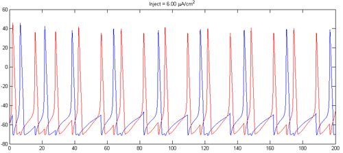
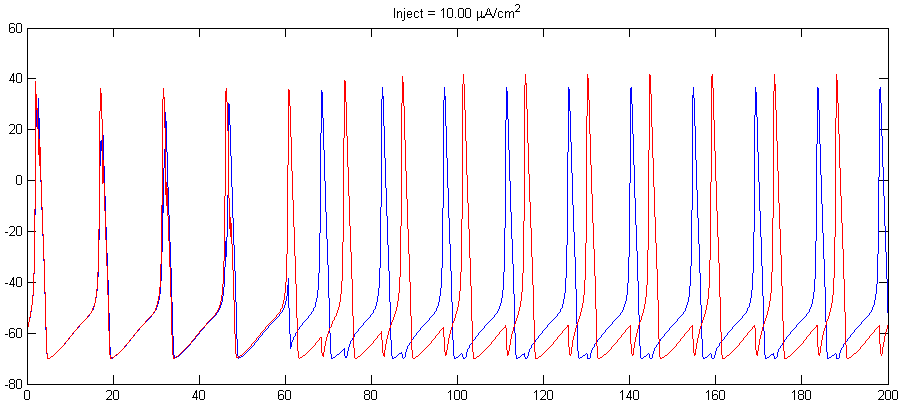
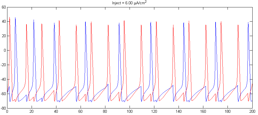
4. Adjust the steady current into the cells and the synaptic strength to make the cells alternately spike as shown below. Consider using inhibitory synapes. Set the steady currents to be slightly different for the two cells. There will be a transient period before phase locking.
   
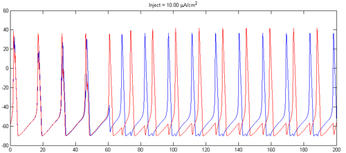
5. Can you find currents and synaptic strengths which causes the cells to fire at 2:1 frequency ratio similarly to that shown below??
   
6. Solution code

5. (Due Tues March 3)

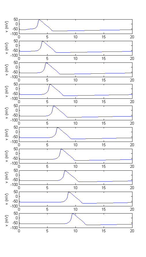
Modify the program, HHpgm1.m, from assignment 4 to support action potential propagation. Use a model for myelinated axons in which each node has HH currents and the between node circuit is a resistor Raxon=1/gaxon representing the axon internal series resistance. The current flowing from node n to the node n+1 is given by I(n,n+1)=gaxon*(Vn-Vn+1) . The net current into a node (entering from the left and leaving to the right) is given by I(n)=gaxon*(Vn-1-Vn)-gaxon*(Vn-Vn+1). There will clearly be special cases for the first and last nodes where no current can enter from the left at node one or leave from the right at the last node.

1. Plot the voltage at each of 10 nodes after an action potential is initiated at the left-most node. Use a specific resistance of 30 ohm-cm for the axonplasm and a diameter of 1.0 mm.
2. Using the diameter given in 1, determine the conduction velocity for at least three different node spacings. How does the conduction velocity depend on node spacing (linear, inverse, inverse squareroot, other)? Does this dependency match the literature?
3. Determine the conduction velocity for at least three different diameters at constant node spacing. Choose a node spacing at which the smallest diameter does not have conduction failure. How does the conduction velocity depend on diameter? Does this dependency match the literature?
4. At what node spacing does propagation fail?

Example plot:

Matlab hints:

• To initialize an entire array
  m = ones(nTime, nNodes).*alpha_m(v-VREST)./(alpha_m(v-VREST)+beta_m(v-VREST));
builds an array with dimension equal to nTime by nNodes. The ".*" and "./" notation means "use per-element operation".
• To address all of the elements in one dimension use ":"
m(i,:) = m(i-1,:) + mdot*DT;
updates the i-th time of all nNodes elements of the array if mdot is a vector of derivitives.
• Solution code

6. (Due Tues March 10)

A 2 to 5 page description of your final project proposal.

7. (Due Tues March 24)

For this assignment we are going to use a somewhat abstract model of neural function invented by Eugene M. Izhikevich. See http://nsi.edu/users/izhikevich/publications/whichmod.htm for much more detail and a matlab program which demos the model. The model simulates the dynamical properties on neurons whithout simulating the ionic properties. This program simulates a neural network with arbitrary synaptic connectivity which you add to and modify below.

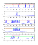
1. Modify the code to simulate the first 5 types of cells with no synaptic connections for 200 mSec. Apply 5 units of current to each cell through the sensory inputs from t=50 to t=100. The plot might look somewhat like the one below. Note that each different type of cell has specific interesting characteristics, such as adaption to a stimulus, or bursting which is modified by input. Do the firing patterns remind you of any of the neurons desribed in class or in the text?
   
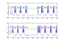
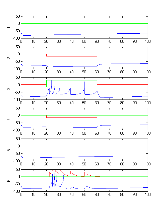
2. Modify the code so that there are two bursting cells (type 3 tonic bursters) synaptically connected so that they fire alternating bursts (like a central pattern generator), but controlled by a sensory stimulus to both cells which stops the firing in both. Run the simulation long enough before and after the sensory input to show phase locking. Perhaps 200 mSec before, 100 mSec during the stimulus, and 200 mSec after (first image below). Extend the stimulus period and the simulation time to show that small sensory inputs can be used to change the pattern period over a range. What is the range of periods, with both positive and negative inputs to both cells?
   
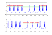
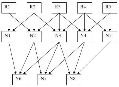
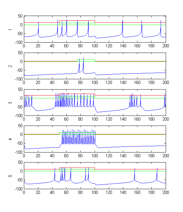
3. Modify the code to make a eight neuron system in which cells 1 to 5 receive sensory input and cell 6 receives the output from cells 1 to 3, and cell 7 receives the output from cells 2 to 4, and cell 8 receives the output from cells 3 to 5. Further more, each of the first 5 cells receives excitatory input from one sensory unit and inhibitory input from the sensory inputs on to each side. (see diagram below). Adjust the synaptic weights from the receptors to the first layer of neurons so that a uniform stimulus produces no output spikes from N1 to N5. Use all type 2 neurons. Adjust the weights between the second and third layers so that a strong edge anyplace in the receptive field produces spikes. Print a few examples. The example output below shows the results of a simulation with just one cell (R6) which receives input from 2 to 4 and with a stimulus centered on the R3.
   

Final Projects

2008

• Simulating the stomatogastric ganglion and the effects of neuromodulators
• A Computational Model for Place Learning in the Hippocampus
• Modeling basic neurobiological concepts
• Understanding magnetic resonance imaging
• An Event Based Neuron Network Model
• Interactive neural simulator

2009

• Exploring a Case of Emergent Synchronization
• Neural Networks and Evolutionary Algorithms
• Central pattern generator/double pendulum model
• A Computational Model for Learning at the Cellular Level
• Computational Hebbian Synapses and Self-Organizing Neural Maps
• Effect of Conductance Changes on the Hermissenda Photoreceptor

Lecture Topics

Possible engineering topics

Introduction: Neuron Hypothesis

How are cells visualized? Technology.
Electrical synapses/close coupling

Introduction to Electrical Signaling in the Nervous System

The nervous system is an electrochemical machine. Neural nets and computation.
Comparison to a digital computer.

Resting Potential

Electrochemical equilibrium, Goldman eqn
Chemistry behind channel specificity
Equivalent circuits, compare to Goldman eqn.

Action Potentials and Propagation I

The transatlantic cable and cable equation.
Need for nonlinear amplifiers.
Equivalent circuits and electronic implementation.

Action Potentials and Propagation II

HH model and simulations
Spiketrain analysis, information theory

Ion Channel Structure, Function, and Diversity

Exponential duration distributions implied from chemistry. Simulation of relation between chemical equations and channel times.

Diseases of Ion Channels (channelopathies)

Quantitative estimates of ionic disturbances, rates, amplitudes, number of channels.
Poisons,Genetics

Ionic Mechanisms of Synaptic Excitation

Electrical synapses/chemical synapses
Equivalent circuits/current flows

Inhibition and Neuronal Integration

Automatic gain control
Nonlinear effects, equvalent circuits

Release of Neurotransmitter

Chemistry of vesicle fusion, diffusion equation, coupled reaction/diffusion

Neuromodulation

Multiple modes of systems of nonlinear oscillators.

Neurochemistry

Just say "know": Drugs and the Brain

Chemical kinetics, enzyme variability

Building Blocks of the Nervous System:
Part 1,2

Control of Movement

Central pattern generation by nonlinear oscillators

Parkinson’s Disease: A Molecular & Personal Perspective

Feedback control systems, stability, lag, delays.

Neural Systems for Sensory Maps

Spike train analysis and information theory

Language and Hemispheric Dominance

Probabilistic inference from sensory data

Sleeping, Dreaming and Waking

Wake/sleep chemical nonlinear oscillator

Emotional Centers of the Brain

Principles of Sensory Function

Statistical problems that sensory systems must solve.

Sensory Transduction

Tunneling? Quantum efficiency. Gain. Cool mechanisms.

Visual Periphery

Image compression, gradient emphasis, lateral inhibition. Spatial aliasing.

Vision in the CNS

Wavelet transform. Redundancy of the average visual scene. Compression in the visual system.

Hearing

Fourier Transform. Impedance matching. Traveling wave on a inhomogeneous membrane.

Sensory Motor Integration

Converting from Cartesian to body-joint coordinates, inverse kinematics

Specification of Neural Tissue I

Specification of Neural Tissue II

The Directed Movement of Neurons and Axons

Chemical kinetics and gradient following

Apoptosis

Neurotropic Factors

Learning & Memory I: non-associative learning

Integrate and fire schemes/neural nets
Pulsed networks vs. Hopfield networks
Equivalent circuit of variable synapse

Learning & Memory II: classical conditioning

Synchrony, stability,

Learning & Memory III: operant conditioning

Complex Learning

Hebbian Learning and LTP
Is LTP involved in learning?

Comparison to back-prop networks
Local normalization requirements
simulation